The code is given in tut2.cpp app11(). The control files which were in action during the production of the video are all copied to the directory t20230918app11 and can be discerned from other runs by the name appendix '_941'. The video shows the relation between the elliptical Kepler orbit (together with the orbiting body, all in blue) and the linear orbit of the Kepler oscillator (together with the oscillating body, all in red). The yellow body (the sun) marks one of the focal points of the Kepler orbit. Notice that the motion of the blue body is determined (up to a factor which is determined by the numerical value of the period) by Kepler's second law of planetary motion and that the motion of the red body is coupled to that of the blue body as by gears.
Let us now discuss the Kepler oscillator in terms of Theoretical Physics of today: We consider two gravitating non-relativistic point masses \(M\) and \(m\) which move around each other. (A symbol associated with a point mass may stand for its mass or for its location (a point) or for both.) This gravitational two-particle problem and its reduction to a one-particle central field problem is well-known; a particularly diligent treatment of the system can be found in Chapter 3 of Herbert Goldstein's classical textbook (e.g. Goldstein Safko Poole: Classical Mechanics, Third edition, Pearson 2014). Here we follow mainly the analysis and the notation of this book with the exception that we introduce at the very beginning the simplifying assumption that \(M\) is much larger than \(m\). This is plausible in the context of Kepler's work where the celestial bodies of interest were the sun and the planets. Due to \( M \gg m \) the position of \(M\) is very close to the center of mass of the two-particle system. Therefore the motion of \(M\) can be ignored and what we perceive is that \(m\) orbits a fixed heavy point mass. For conveniece we chose the location of \(M\) as 'the origin' in our definition of position vectors \(\mathbf{r}\). Then the force which \(M\) exerts on \(m\) is \(-k\frac{\mathbf{r}}{r^3}\), where \(k := G M m \) with \(G\) denoting Newton's gravitational constant.
The most convenient way to describe the motion of \(m\) is by giving the Lagrangian
$$ L = \frac{m}{2} \dot{\mathbf{r}}^2 + \frac{k}{r}\,\,. \quad (1)$$ This is a three-dimensional system in the sense that the set of all trajectories (orbits) fills the three-dimensional space. However, each single orbit is contained in a plane. This plane is determined by the condition that it contains \(M\) and is perpendicular to the axial vector \( \mathbf{r} \times \dot{\mathbf{r}} \), where \( \mathbf{r} \) points to an arbitrary point of the orbit. Given this plane and the origin we can select an arbitrary system of polar coordinates with respect to the origin. The orbit then is described by giving polar coordinates \( r \) and \( \varphi \) as functions of time \( t \). Expressing the Lagrangian in terms of these polar coordinates we get $$ L = \frac{m}{2}(\dot{r}^2 + r^2 \dot{\varphi}^2) + \frac{k}{r}\,\,. \quad (2)$$ Since we have only two 'dynamical variables' (namely \(r\) and \(\varphi\)) we now deal with a dynamical system with two degrees of freedom. One should recognize that we got to this system by natural manipulations (actually by exploiting that the vector of angular momentum is a constant of motion) on a system with 3 degrees of freedom given by the coordinates \(r_1, r_2, r_3\). Both systems have the same Lagrangian \(L\) according to our notation.
This shows that \(L\) is not treated as a function in the elementary sense in which functions are used in modern mathematical presentations of the calculus. Objects with the semantics of the physicist's \(L\) occur in mathematics only since the introduction of differential manifolds. Here they correspond to 'scalar' functions on the underlying set \( \mathcal{B}\) (on which an 'atlas' is given as a set of chart-functions). Theoretical physicists traditionally don't define \( \mathcal{B}\); they rely on coordinates which are supposed to be measurable 'in the real world' and which give rise to numerical chart-functions, if a system of primary coordinates ('ur-coordinates') is supposed to be given. For a computational treatment it is very convenient to start from a description in terms of numerical functions. Mathematical physicists, by contrast, normally avoid working with coordinates. The price for this is, as a rule, strongly reduced readability and less guidance for creating numerical models.
Now we obtain the two Lagrange equations from (2): $$ \frac{d}{dt} \frac{\partial}{\partial \dot{r}} L - \frac{\partial}{\partial r} L= m \ddot{r} + m r \dot{\varphi}^2 - \frac{k}{r^2} = 0\,\,. \quad (3)$$ $$ \frac{d}{dt} \frac{\partial}{\partial \dot{\varphi}} L = \frac{d}{dt} m r^2 \dot{\varphi}= 0\,\,. \quad (4)$$ Equation (4) says that the quantity \(m r^2 \dot{\varphi} \), which obviously equals the modulus of the orbital angular momentum of \(m\) is a constant of motion. We denote this constant value by \( l \). Inserting \(m r^2 \dot{\varphi}\) in (2) we eliminate the variable \(\varphi\) (as is always possible with cyclic variables) and obtain the equation
$$m \ddot{r} = \frac{l^2}{m r^3} - \frac{k}{r^2}\,\,, \quad (5) $$ in which the modulus \(l\) of the angular momentum appears as a parameter on par with the parameters \(m\) and \(k\). We have obtained an equation of motion for a mechanical system with only one degree of freedom. To fully appreciate the nature of this system we give its Lagrangian and its Hamiltonian. Equation (5) is easily shown to be the Lagrange equation of the following Lagrangian $$ L = \frac{m}{2} \dot{r}^2 + \frac{k}{r} - \frac{l^2}{2 m r^2}\,\,. \quad (6)$$ And from the Lagrangian (6) we obtain the Hamiltonian $$ H = \frac{ p^2}{2 m} - \frac{k}{r} + \frac{l^2}{2 m r^2}\,\,. \quad (7)$$
By choosing suitable units for time, length, and mass we can give all three parameters the numerical value 1 so that we get a an equation which is free of parameters - just as for the equations of the harmonic oscillator when the Hamiltonian is written as \(\frac{1}{2}(p^2 + q^2)\). For this to work we have to assume that \(l \neq 0\). In doing so we only omit the simple and unrealistic case of collision orbits. It might be entertaining to find the normalizing units mentioned above in a concrete example, e.g. for the orbit of the Earth around the Sun: Here the units come out as 171.3 s, 8.74 108 m (72% of the mean distance between Earth and Moon), and 5.97 1024 kg (Earth's mass). The corresponding numbers for Mars are 218.5 s, 1.07 109 m, 6.42 1023 kg.
This elimination of the parameters \(m, k, l\) turns the Hamiltonian (7) into the following numerical function (suitable for programming): $$ H(v,x) := T(v) + V(x) := \frac{1}{2} v^2 + \frac{1}{x} \Bigl(\frac{1}{2x}-1\Bigr), \quad \frac{1}{2} < x < \infty\,\,, \quad \quad (8)$$ where we have written \(v\) and \(x\) for what in the context of general Hamiltonian theory would be written as \(p\) and \(q\). (Notice that we enforced \(m = 1\) so that \(p = v\) is natural). The Hamiltonian formulation of equations of motion has the advantage that it gives not only expressions for \(\dot p\) and \(\dot q\) but also a closed expression for an constant of motion: the function \(H\) itself. This means that the value \(H(v(t),x(t))\) is independent of \(t\) for any trajectory. This constant value, let us denote it by \(h\), has the physical meaning of the total energy of the oscillator. It lies in the interval \([-1/2,0)\) if the trajectory is bounded and in \([0, \infty)\) otherwise. Here, we are only interested in the bounded case (i.e. \(h < 0\)). Then the solution of the corresponding central force problem (see above) is an ellipse with a numerical eccentricity (eccentricity for short) (\(\epsilon = \sqrt{1+2h}\). For the smallest possible value \(h=-\frac{1}{2}\) the eccentricity comes out as \(0\), so that the corresponding ellipse is a circle. For the large semi-axis \(a\) of the corresponding ellipse we have $$ a = \frac{1}{1-\epsilon^2}\quad, $$ and for the period \(t_P\) $$ t_P = 2 \pi a^{\frac{3}{2}} \quad. $$ The one-dimensional mechanical system described by the Hamiltonian (8) is what we refer to as Kepler oscillator due to its close relation to the radial motion associated with Kepler orbits.
From the viewpoint of numerical analysis the most important property of the Kepler oscillator is that for arbitrary initial conditions the state for any point \(t\) in time can be computed to any given accuracy within a time independent of \(t\) by iteratively solving an transcendental equation known as Kepler's equation. Further, it is arguably the least trivial system having this property. Therefore this dynamical system was chosen as the prominent test system in An asynchronous leapfrog method II (Nov 2013, 14 MB, http://www.arxiv.org/abs/1311.6602). It is to be noted, however, that in one respect the Kepler oscillator is rather special: As a Hamiltonian system it is separable and as system of Newtonian mechanics, its force term does not depend on the velocity. The present study extends some of the visualizations in this reference by replacing still images by motion pictures. This turns out to be particularly interesting for what was introduced in the reference as the numerical interaction picture associated with numerical integrators for dynamical systems.
The following video shows the motion of the oscillator particle in a position-energy diagram for 7 values of the numerical eccentricity \(\epsilon\). The potential \(V\) in (8) shows up as the asymmetrical curve from which a large part can be seen in the video. Depending on the total energy (which is constant along each trajectory) of the oscillator particle, it oscillates between a minimal and a maximal position x. For a proper understanding of the parameters in the diagrams and in the ini-files it is good to note that \(\epsilon\) parameterizes the orbits, whereas \(E\) parameterizes positions in an orbit. As was explained earlier in detail, the motion of the Kepler oscillator particle is just the radial motion in a Kepler orbit. It is this corresponding motion in a Kepler orbit to which the quantities \(\epsilon\) and \(E\) refer directly.
The code is given in tut2.cpp app10(). The control files which were in action during the production of the video are all copied to the directory t20230919app10 and can be discerned from other runs by the name appendix '_512'. This shows the potential \(V\) in (8) over the x-range which is needed to represent the orbit for \(\epsilon = 0.7\). The closer \(\epsilon\) comes to 1, the larger the x-range needed to represent the whole trajectory of the oscillator particle. We see that the period grows with growing \(\epsilon\). For two periods of the upper state, the first state above the lowest state does some 5.5 periods. Unlike the harmonic oscillator, the Kepler oscillator shows a decreasing frequency for increasing amplitude.
In the present study we view the Kepler Oscillator as a system of classical mechanics. Of course, it can be viewed as a quantum mechanical system as well. In this respect we have the same situation as for the harmonic oscillator. All the numerical integrators considered here can also be used to simulate the dynamics of the quantum mechanical Kepler oscillator. Actually, the asynchronous leapfrog integrators where invented for simulating quantum dynamics. The reason for the present restriction to the classical version is that here simpler and clearer quantitative criteria for errors of numerical methods are available:
All trajectories are strictly periodic in exact dynamics and not necessarily so in simulations by integrators. The period is given by a simple explicit formula in terms of the initial state.
The deviation of a simulated state from the exact state can be computed to arbitrarily fixed accuracy in constant time.
Symplecticity of an integrator is easily checked when applied to classical trajectories and arguably not so for quantum trajectories.
A.1. Two numerical integrators compared with the exact solution.
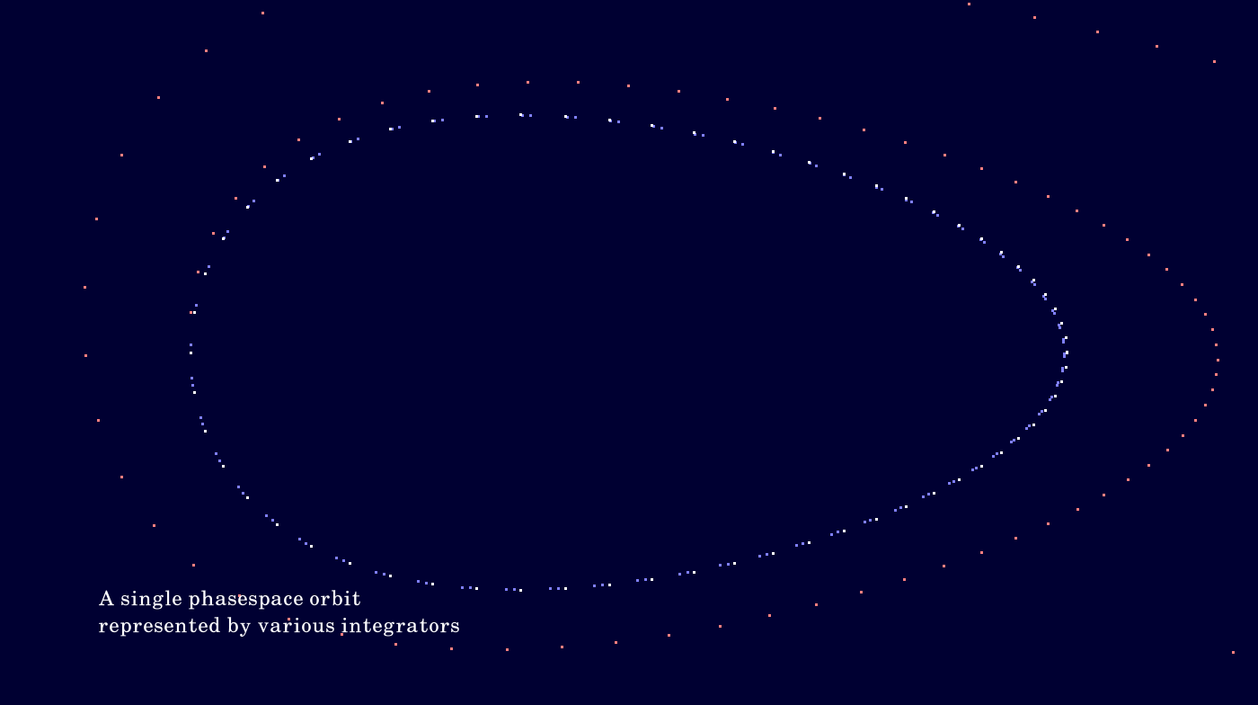
Besides the 1-dimensional motion of the oscillator particle in position space there is a 2-dimensional motion in the corresponding phase space. This gives rise to a phase space diagram (also known as 'phase space orbit' and 'phase portrait'). In the next image we see such an phase space orbit belonging to \(\epsilon = 0.25\) as simulated with the numerical integrator Euler (red), the numerical integrator LF (original leapfrog, blue), and with exact dynamics (white). For numerical integrators the time step size is an important parameter. Here it is chosen as \(\frac{1}{64}\) of the period, which amounts at a rather coarse sampling of the quite asymmetric orbit. So it comes without surprise that the simple Euler integrator fails to follow the orbit to any reasonable degree of accuracy. The leapfrog integrator gives positions that deviate from the correct positions not noticeably in lateral direction but move noticeable too fast along the orbit. The pattern of the blue points clearly shows that the simulation shows two complete periods. The essential observation later will be that the asynchronous leap frog algorithms are considerably more accurate than the original leap frog integrator.
The code is given in tut2.cpp app1(). The control files which were in action during the production of the video are all copied to the directory t20230911app1 and can be discerned from other runs by the name appendix '_240'. There are shown two revolutions of the oscillator particle (nPerRev=64, nRev=2 see file app1_240.ini)
A.2. All the integrators considered here in action on the orbit from A.1.
In the next image the number of revolutions is increased from 2 to 40 and instead of only 3 integrators, all 10 integrators implemented in project tut2 are shown.
How numbers and colors are associated with integrator methods:
\(\quad\) 1 Euler LIGHTRED
\(\quad\) 2 RK2 (Runge Kutta 2nd order) ORANGE
\(\quad\) 3 DMI (direct midpoint integrator) LIGHTGREEN
\(\quad\) 4 ALF (asynchronous leap frog) GREEN
\(\quad\) 5 DALF (densified asynchronous leapfrog) CYAN
\(\quad\) 6 LF (original leap frog) BLUE
\(\quad\) 7 ADALF (averaged densified asynchronous leap frog) MAGENTA
\(\quad\) 8 AALF (averaged asynchronous leap frog) FAINTGRAY
\(\quad\) 9 HAM (Hamilton, symplectic Euler) LIGHTGRAY
\(\quad\) 10 Exc (exact) WHITE
Only the 'green blue methods' (lightgreen, green, cyan, blue) follow the exact orbit with reasonable accuracy.
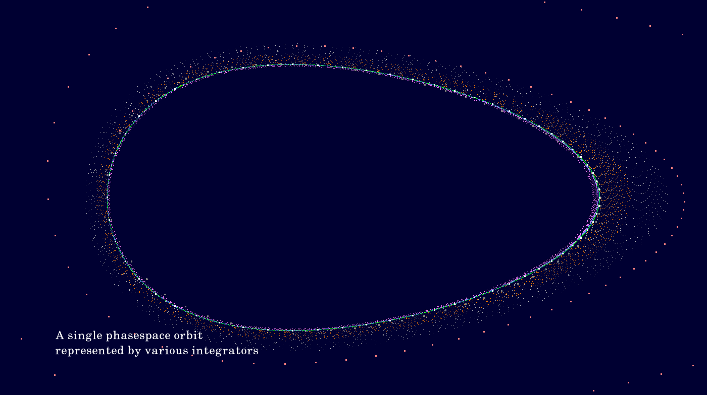
The code is given in tut2.cpp app1(). The control files which were in action during the production of the video are all copied to the directory t20230912app1 and can be discerned from other runs by the name appendix '_223'. There are shown 40 revolutions of the oscillator particle (nPerRev=64, nRev=40 see file app1_223.ini)
B.1. Exact solution compared with asynchronous leapfrog integrator.
The code is given in tut2.cpp app2(). The control files which were in action during the production of the video are all copied to the directory t20230812b and can be discerned from other runs by the name appendix '_819'. This video shows a content similar to that of the second video (please discern images and videos), however, in a form that is quite different. What shown is not the motion along an orbit, but the orbit itself. Not as energy versus \(x\), but as \(x\) versus \(v\) thus as an orbit in phase space. The quantity that changes its value from video frame to video frame is the eccentricity of the orbit: it grows from 0.1 to 0.25 in 200 steps. Actually, we see not only the exact orbit but the exact orbit overlayed with the orbit as represented by use of the numerical integrator ALF. For each of the selected eccentricities two full orbital periods are drawn, where 40 positions are computed for each period (which means that the time-step with which the numerical integrator is called grows with the eccentricity. and thus from frame to frame). What the video shows is that the asynchronous leapfrog integrator computes orbits that can't be discerned from the exact ones at the given graphical resolution.
B.2. Runge-Kutta 2nd order inferior to leap frog.
The code is given in tut2.cpp app2(). The control files which were in action during the production of the video are all copied to the directory t20230812d and can be discerned from other runs by the name appendix '_522'. This is similar to the foregoing video. What is shown is the orbit as represented by the Runge Kutta inegrator RK2. The exact orbit is not given and for each orbital period the eccentricity grows from 0.1 to 0.4 in 200 steps. For each of the selected eccentricities 3 full orbital periods are drawn. All other numbers given for the previous video apply for the present one as well. The video clearly shows that the computed orbits don't repeat exactly: the 3 revolutions that are drawn for each of the 200 selected eccentricities can easily be separated visually. Both, ALF and RK2, are second order explicit integrators. Nevertheless they are quite different in their ability to represent the orbit accurately.
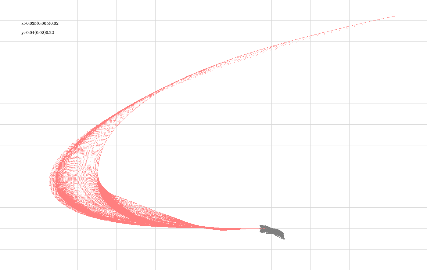
C.1. 'Best and worst' for second order integrators
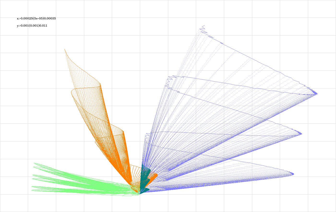
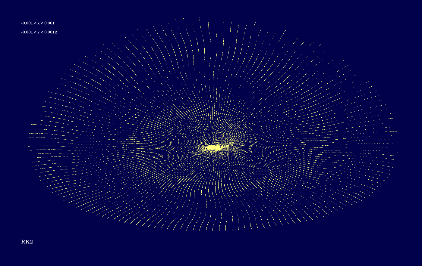
The code is given in tut2.cpp app2(). The control files which were in action during the production of the video are all copied to the directory t20231007app2_12e. The parameter which varies from video frame to video frame is the eccentricity. If grows from 0.1 to 0.4 in 200 steps. For any selected value of \(\epsilon\), 80 states are computed for each integrator from the list {RK2, DALF}, and for each of the 3 revolutions. This shows the orbit as interaction picture for the 'best' and the 'worst' of the integrators of second order. Notice that a long trajectory in this type of visualization means large error of the numerical integrator.
The above image shows the superposition of all trajectories occurring in the video. The data for this frame were computed in a first step of 'video production' to find the window in object space which will be large enough to show all frames of the video without an adjustment of scale during the 'show'. As it occurred very often to me a data set which was created for some program-internal reason turned out to look quite interesting as a graphics. So I include this (and similar ones later) graphics 'for entertainment'.
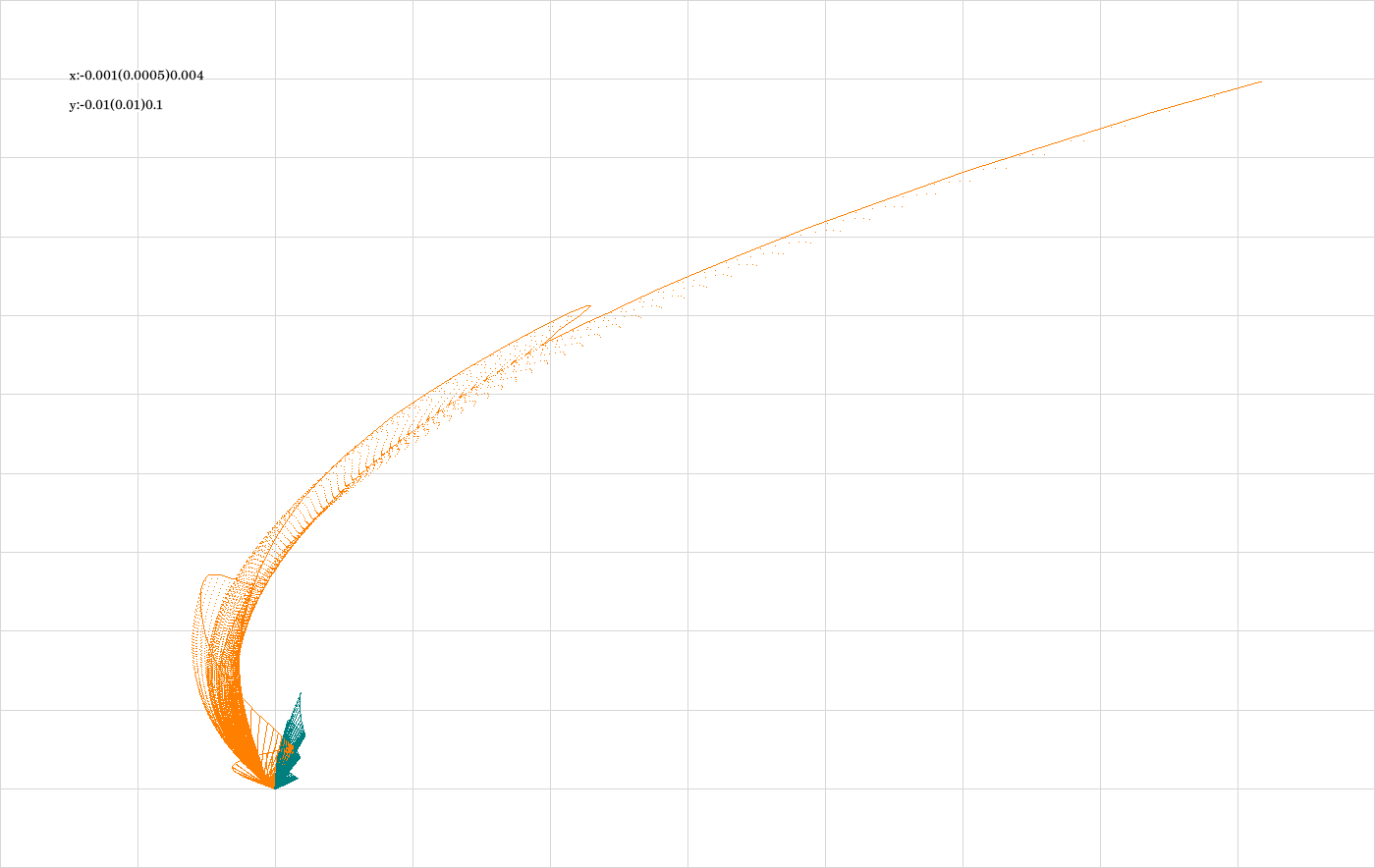
C.2. 'Best and worst' for first order integrators
Same topic as in C.1. but with different integrators.
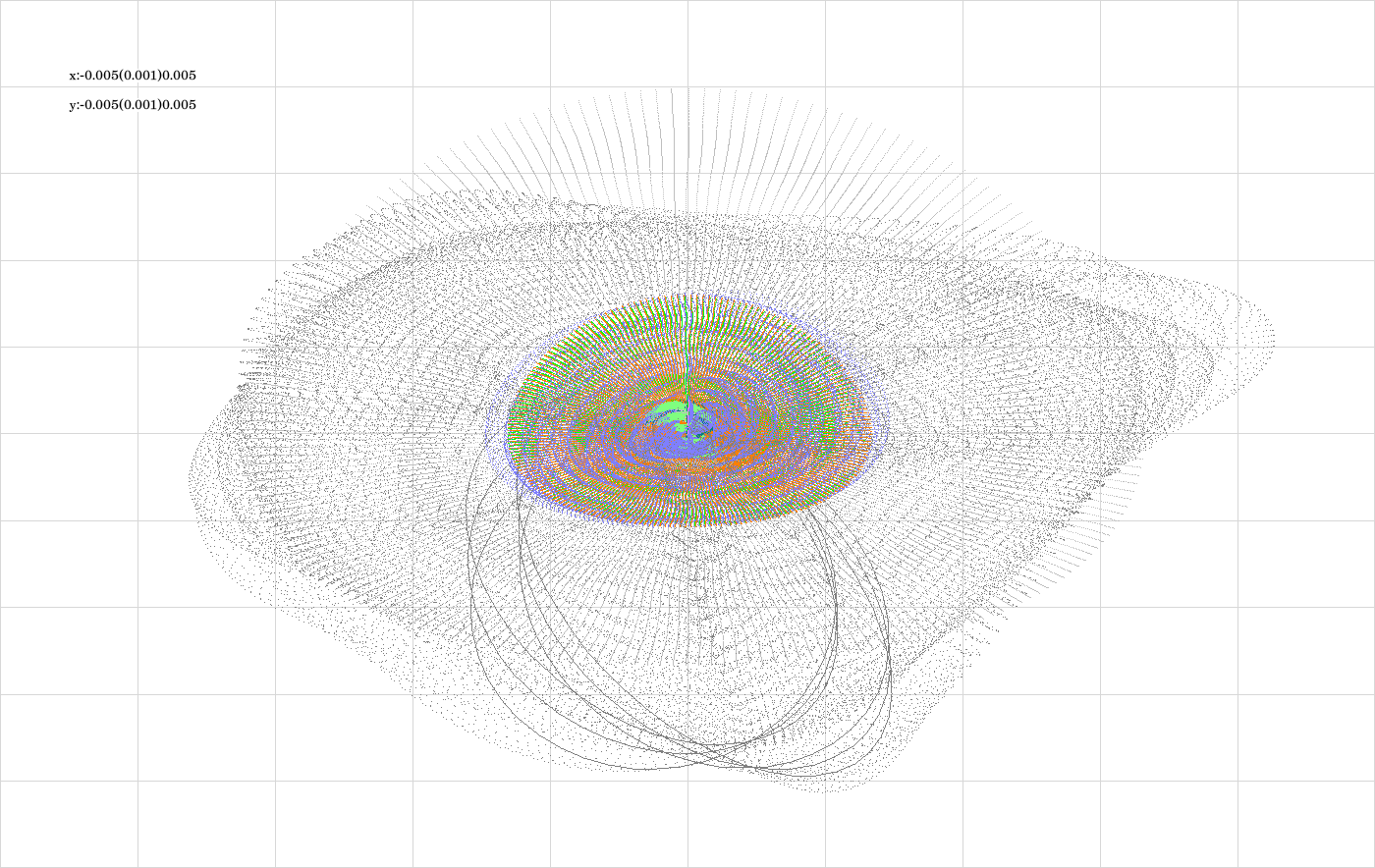
The code is given in tut2.cpp app2(). The control files which were in action during the production of the video are all copied to the directory t20231003app2_firstOrd. The parameter which varies from video frame to video frame is the eccentricity. If grows from 0.1 to 0.4 in 200 steps. For any selected value of \(\epsilon\), 80 states are computed for each integrator from the list {Euler, HAM}, and for each of the 3 revolutions. This shows the orbit as interaction picture for the well-known Euler integrator (which is for teaching only) and its symplectic cousin (which can be coded even slightly simpler as the non-symplectic original). I found this integrator as formula (10.2) in the book J.M.Sanz-Serna and M.P. Calvo: Numerical Hamiltonian Problems. There it is classified as the 'first-order symplectic partitioned Runge-Kutta method (1)[1]'. Curiously one has there to evaluate the second equation prior to the first one to get an explicit algorithm.
The above image shows the superposition of all trajectories occurring in the video (see comment to the previous image).
C.3. Diversity in second order integrators
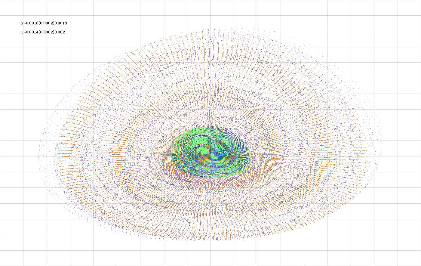
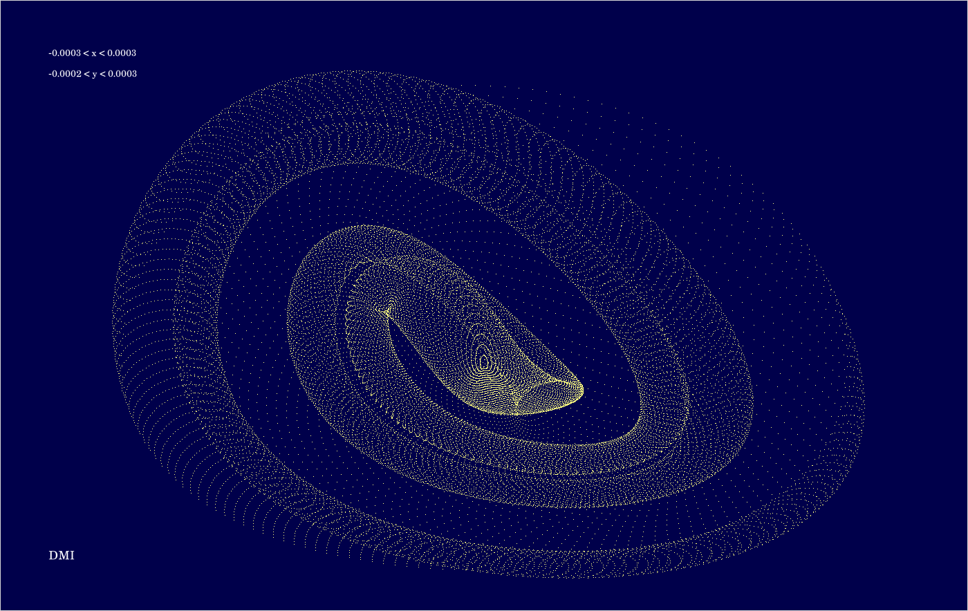
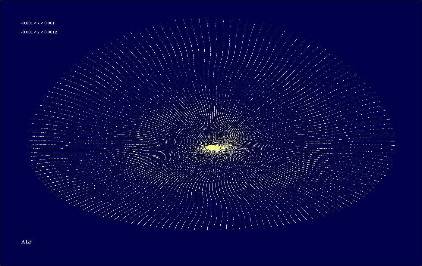
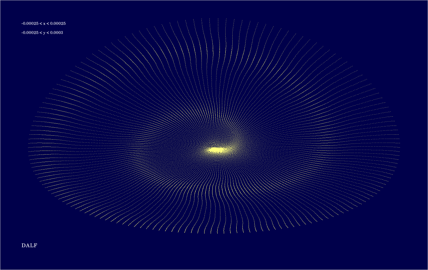
The code is given in tut2.cpp app2(). The control files which were in action during the production of the video are all copied to the directory t20231001app2_12f. The parameter which varies from video frame to video frame is the eccentricity. If grows from 0.1 to 0.25 in 200 steps. For any selected value of \(\epsilon\), 100 states are computed for each integrator from the list {RK2, DMI, DALF, LF}, and for each of the 3 revolutions. The intention here is to include the integrators of second order which produce in this type of visualization the most interesting geometry.
The above image shows the superposition of all trajectories occurring in the video (see comment to the previous image).
D.1. All integrators (except for Euler)
The code is given in tut2.cpp app2(). The control files which were in action during the production of the video are all copied to the directory t20231007app2_12g2. Now \(\epsilon\) has the fixed value 0.1. The parameter which varies from video frame to video frame is the eccentric anomaly \(E\). If grows from 0 to 6.28 in 200 steps. For any selected value of \(E\), 100 states are computed for each integrator from the list {RK2, DMI, ALF, DALF, LF, ADALF, AALF, HAM}, and for each of the 3 revolutions.
The above image shows the superposition of all trajectories occurring in the video (see comment to the previous image).
D.2. Selection for better resolution
The code is given in tut2.cpp app2(). The control files which were in action during the production of the video are all copied to the directory t20231007app2_12g.Now \(\epsilon\) has the fixed value 0.1. The parameter which varies from video frame to video frame is the eccentric anomaly \(E\). If grows from 0 to 6.28 in 200 steps. For any selected value of \(E\), 100 states are computed for each integrator from the list {RK2, DMI, DALF, LF}, and for each of the 3 revolutions. For the small eccentricity chosen here the RK2-trajectory is approximately as long as the LF-trajectory. For more resolutions and larger eccentricity it would outgrow all 3 others drastically.
The above image shows the superposition of all trajectories occurring in the video (see comment to the previous image).
E.1. Integrator Euler
The code is given in tut2.cpp app2(). The control files which were in action during the production of the video are all copied to the directory t20231004app2_single1. The parameter which varies from video frame to video frame is the eccentric anomaly \(E\) of the initial state. If grows from 0 to \(2 \pi \) in 200 steps. For any of the selected values of \(E\), 100 states are computed for each of the 2 revolutions.
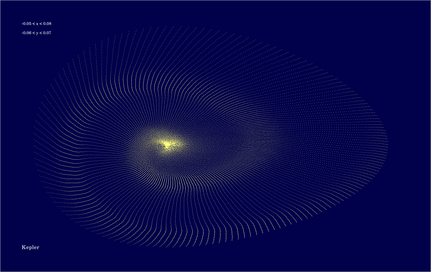
The above image shows the superposition of all trajectories occurring in the video (for entertainment as explained earlier).
E.2. Integrator RK2
The code is given in tut2.cpp app2(). The control files which were in action during the production of the video are all copied to the directory t20231004app2_single2. The parameter which varies from video frame to video frame is the eccentric anomaly \(E\) of the initial state. If grows from 0 to \(2 \pi \) in 160 steps. For any of the selected values of \(E\), 100 states are computed for each of the 2 revolutions.
The above image shows the superposition of all trajectories occurring in the video (for entertainment as explained earlier).
E.3. Integrator DMI
The code is given in tut2.cpp app2(). The control files which were in action during the production of the video are all copied to the directory t20231004app2_single3. The parameter which varies from video frame to video frame is the eccentric anomaly \(E\) of the initial state. If grows from 0 to \(2 \pi \) in 160 steps. For any of the selected values of \(E\), 100 states are computed for each of the 2 revolutions.
The above image shows the superposition of all trajectories occurring in the video (for entertainment as explained earlier).
E.4. Integrator ALF
The code is given in tut2.cpp app2(). The control files which were in action during the production of the video are all copied to the directory t20231004app2_single4. The parameter which varies from video frame to video frame is the eccentric anomaly \(E\) of the initial state. If grows from 0 to \(2 \pi \) in 160 steps. For any of the selected values of \(E\), 100 states are computed for each of the 2 revolutions.
The above image shows the superposition of all trajectories occurring in the video (for entertainment as explained earlier).
E.5. Integrator DALF
The code is given in tut2.cpp app2(). The control files which were in action during the production of the video are all copied to the directory t20231004app2_single5. The parameter which varies from video frame to video frame is the eccentric anomaly \(E\) of the initial state. If grows from 0 to \(2 \pi \) in 160 steps. For any of the selected values of \(E\), 100 states are computed for each of the 2 revolutions.
The above image shows the superposition of all trajectories occurring in the video (for entertainment as explained earlier).
E.6. Integrator LF
The code is given in tut2.cpp app2(). The control files which were in action during the production of the video are all copied to the directory t20231004app2_single6. The parameter which varies from video frame to video frame is the eccentric anomaly \(E\) of the initial state. If grows from 0 to \(2 \pi \) in 160 steps. For any of the selected values of \(E\), 100 states are computed for each of the 2 revolutions.
The above image shows the superposition of all trajectories occurring in the video (for entertainment as explained earlier).
E.7. Integrator ADALF
The code is given in tut2.cpp app2(). The control files which were in action during the production of the video are all copied to the directory t20231004app2_single7. The parameter which varies from video frame to video frame is the eccentric anomaly \(E\) of the initial state. If grows from 0 to \(2 \pi \) in 160 steps. For any of the selected values of \(E\), 100 states are computed for each of the 2 revolutions.
The above image shows the superposition of all trajectories occurring in the video (for entertainment as explained earlier).
E.8. Integrator AALF
The code is given in tut2.cpp app2(). The control files which were in action during the production of the video are all copied to the directory t20231004app2_single8. The parameter which varies from video frame to video frame is the eccentric anomaly \(E\) of the initial state. If grows from 0 to \(2 \pi \) in 160 steps. For any of the selected values of \(E\), 100 states are computed for each of the 2 revolutions.
The above image shows the superposition of all trajectories occurring in the video (for entertainment as explained earlier).
E.9. Integrator HAM
The code is given in tut2.cpp app2(). The control files which were in action during the production of the video are all copied to the directory t20231004app2_single9. The parameter which varies from video frame to video frame is the eccentric anomaly \(E\) of the initial state. If grows from 0 to \(2 \pi \) in 160 steps. For any of the selected values of \(E\), 100 states are computed for each of the 2 revolutions.
The above image shows the superposition of all trajectories occurring in the video (for entertainment as explained earlier).
From now on we give no links to ini-files, since the relevant ini-file can be found as app*.ini in the directory to which 'docu-directory' points.
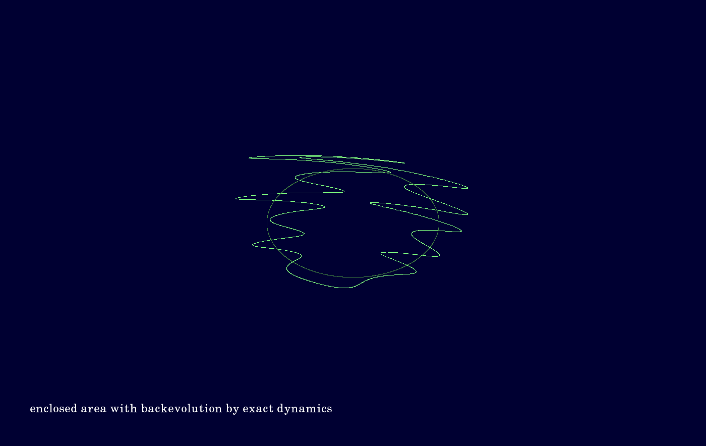
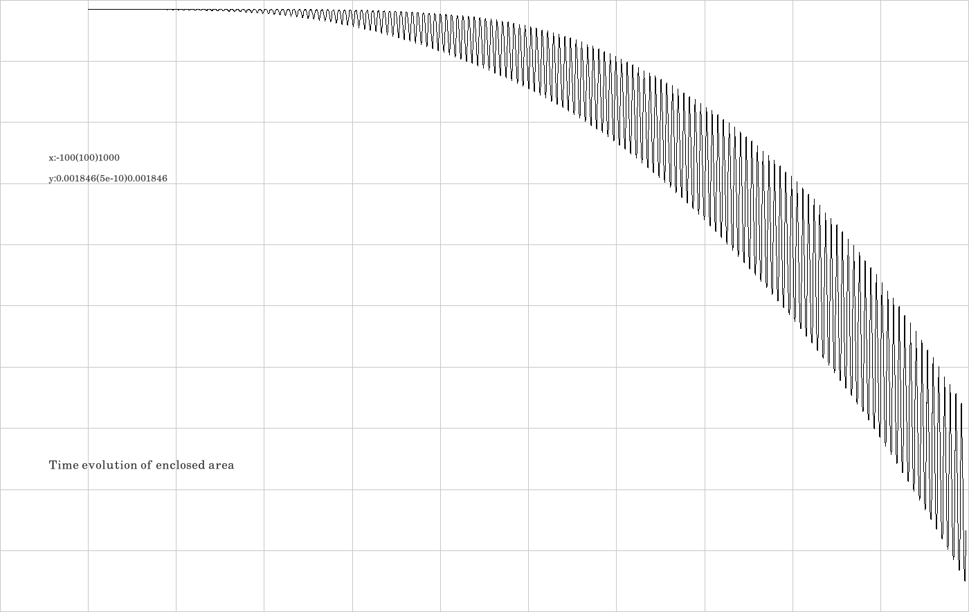
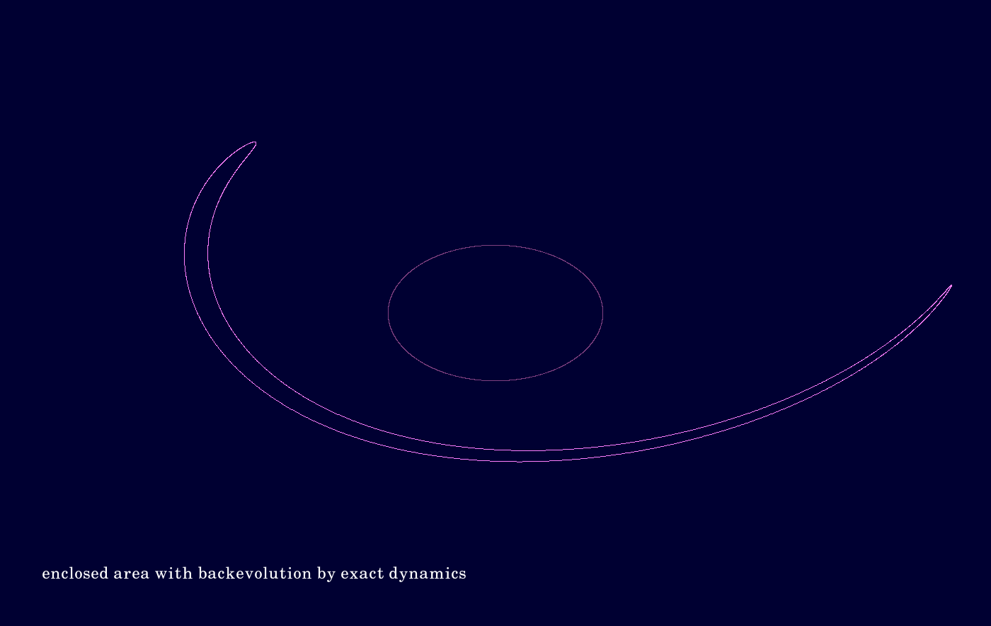
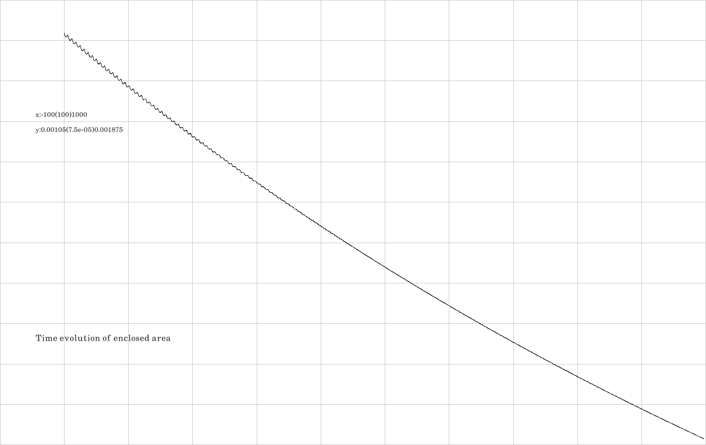
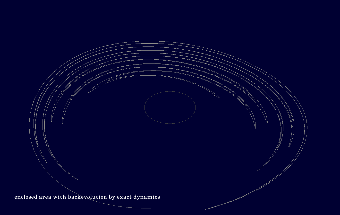
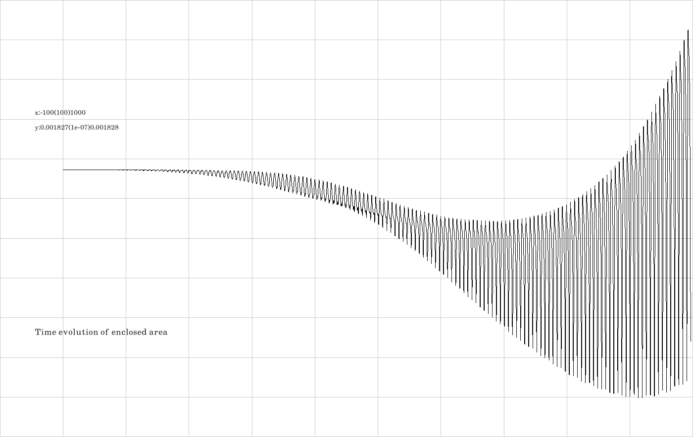
F.1. Integrator Euler
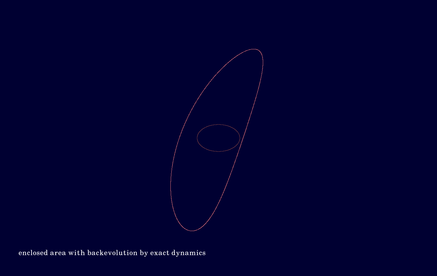
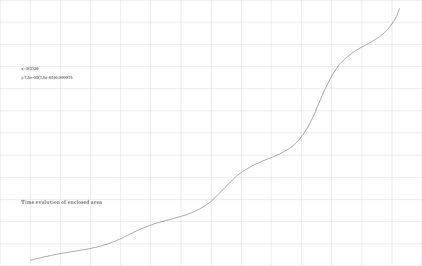
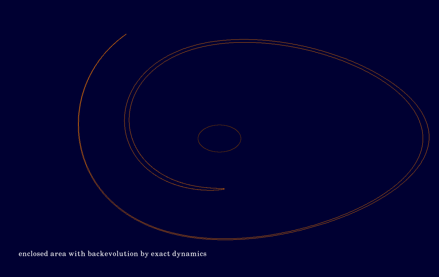
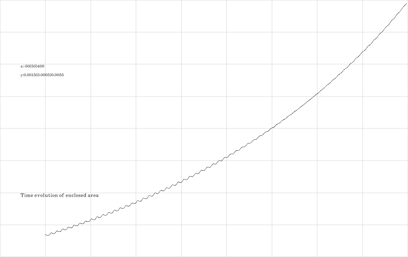
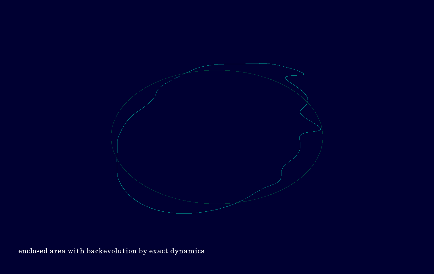
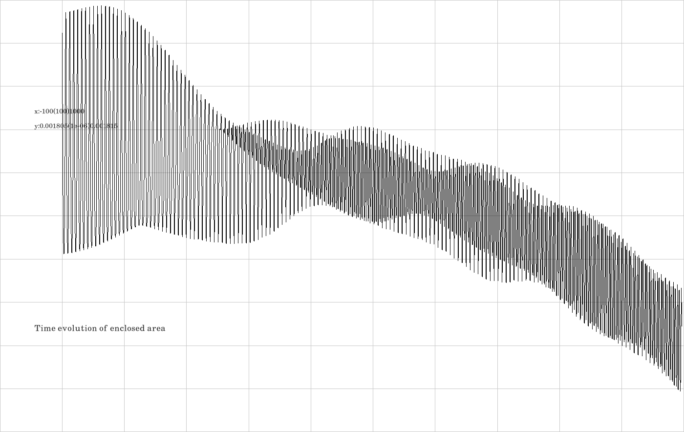
The code is given in tut2.cpp app3(). The control files which were in action during the production of the video are all copied to the directory t20230926app3Euler. The first (dark) image shows the initial and the final contour in the numerical interaction picture of the Euler integrator. One sees that the area within the contour became much larger in the course of time evolution. The second
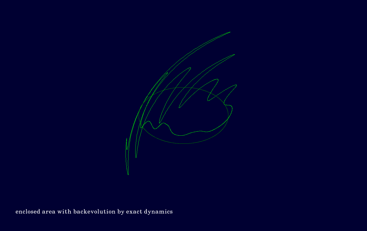
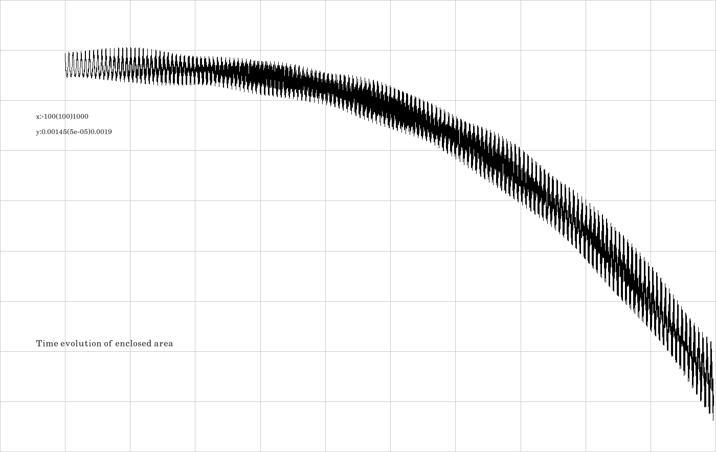
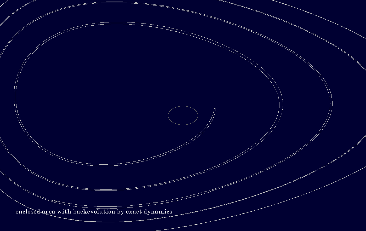
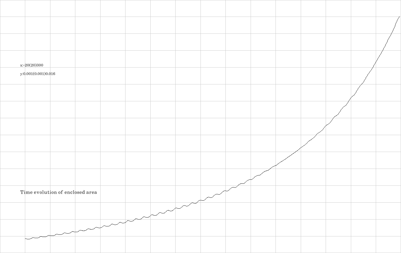
F.2. Integrator RK2
The code is given in tut2.cpp app3(). The control files which were in action during the production of the video are all copied to the directory t20230926app3RK2.
F.3. Integrator DMI
The code is given in tut2.cpp app3(). The control files which were in action during the production of the video are all copied to the directory t20230926app3DMI.
F.4. Integrator ALF
The code is given in tut2.cpp app3(). The control files which were in action during the production of the video are all copied to the directory t20230926app3ALF.
F.5. Integrator DALF
The code is given in tut2.cpp app3(). The control files which were in action during the production of the video are all copied to the directory t20230926app3DALF.
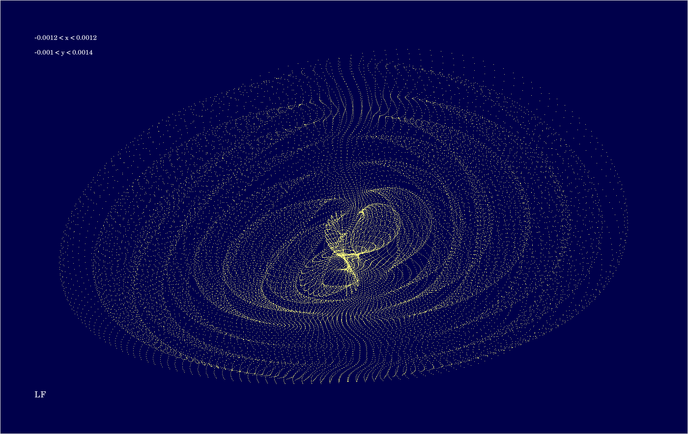
F.6. Integrator LF
The code is given in tut2.cpp app3(). The control files which were in action during the production of the video are all copied to the directory t20230923app3LF.
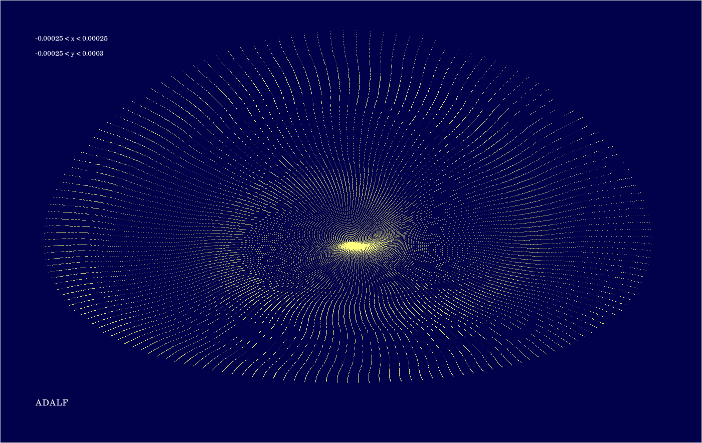
F.7. Integrator ADALF
The code is given in tut2.cpp app3(). The control files which were in action during the production of the video are all copied to the directory t20230926app3ADALF.
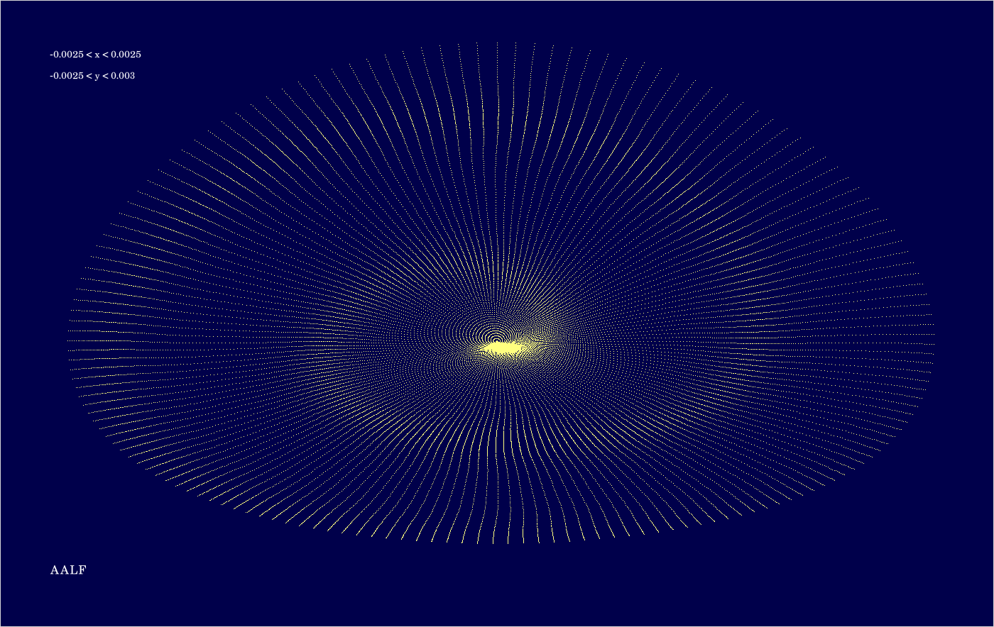
F.8. Integrator AALF
The code is given in tut2.cpp app3(). The control files which were in action during the production of the video are all copied to the directory t20230926app3AALF.
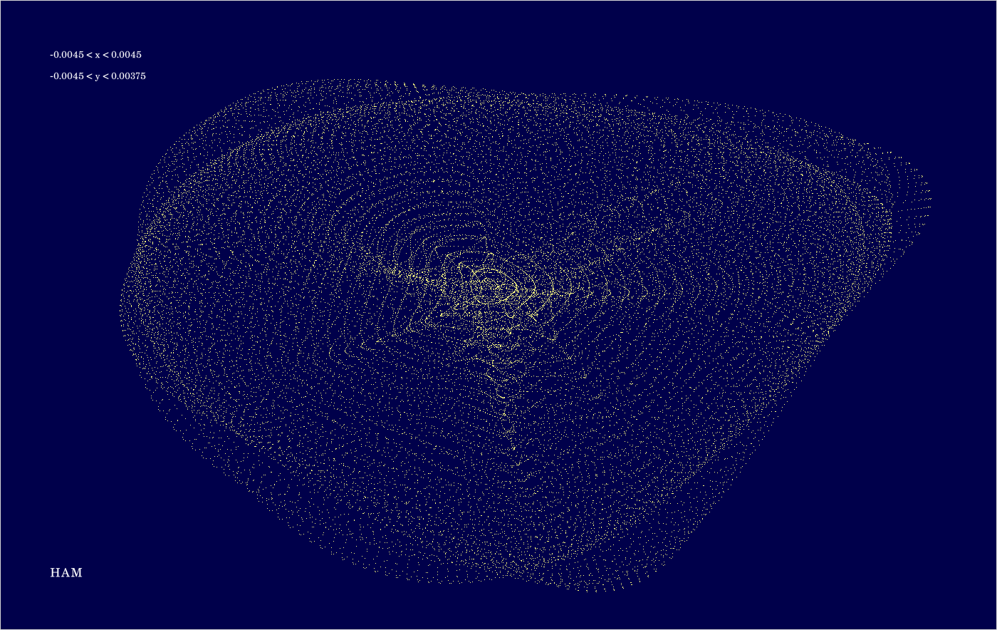
F.9. Integrator HAM
The code is given in tut2.cpp app3(). The control files which were in action during the production of the video are all copied to the directory t20230926app3HAM.
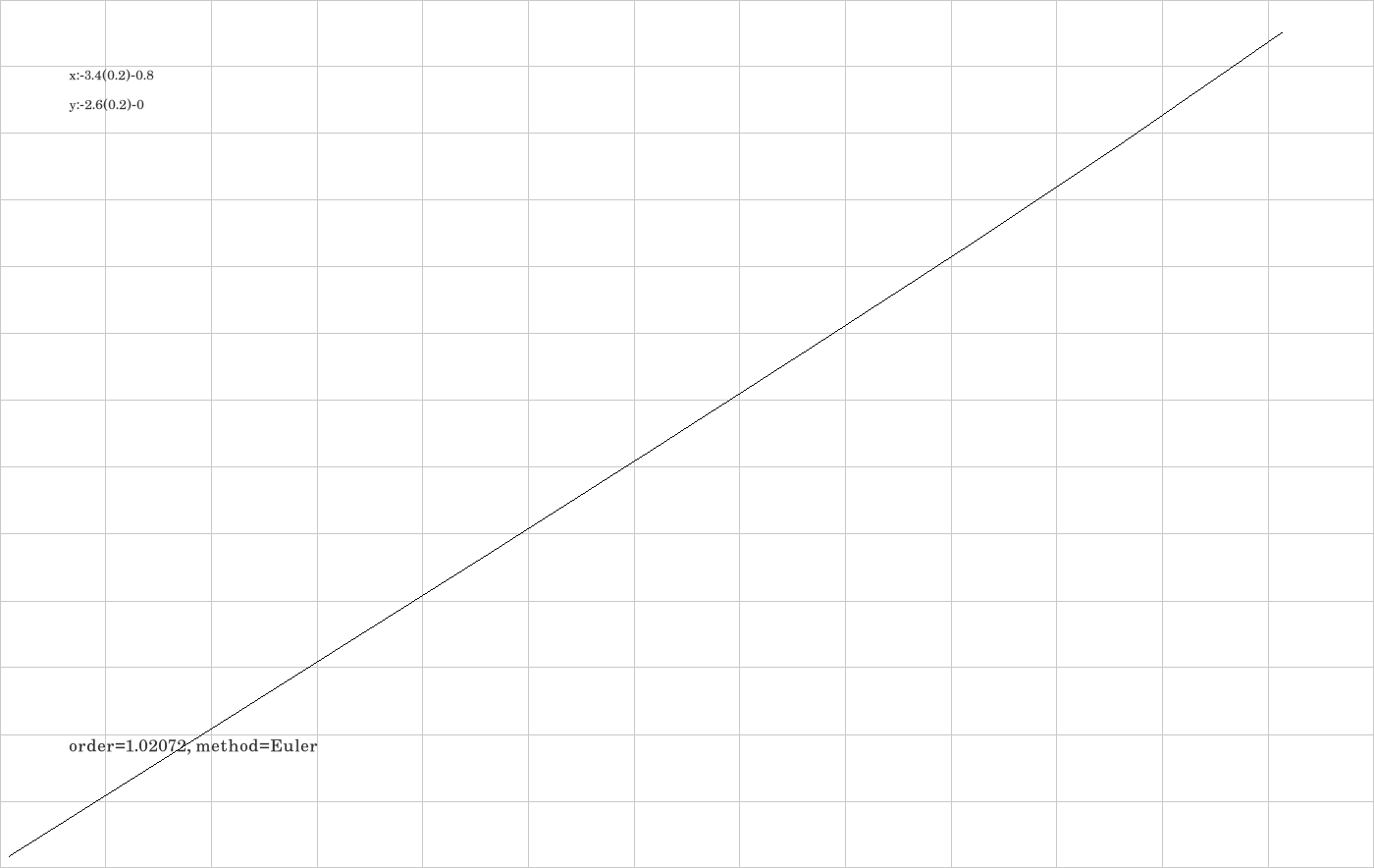
G.1. Empirical order of the Euler integrator
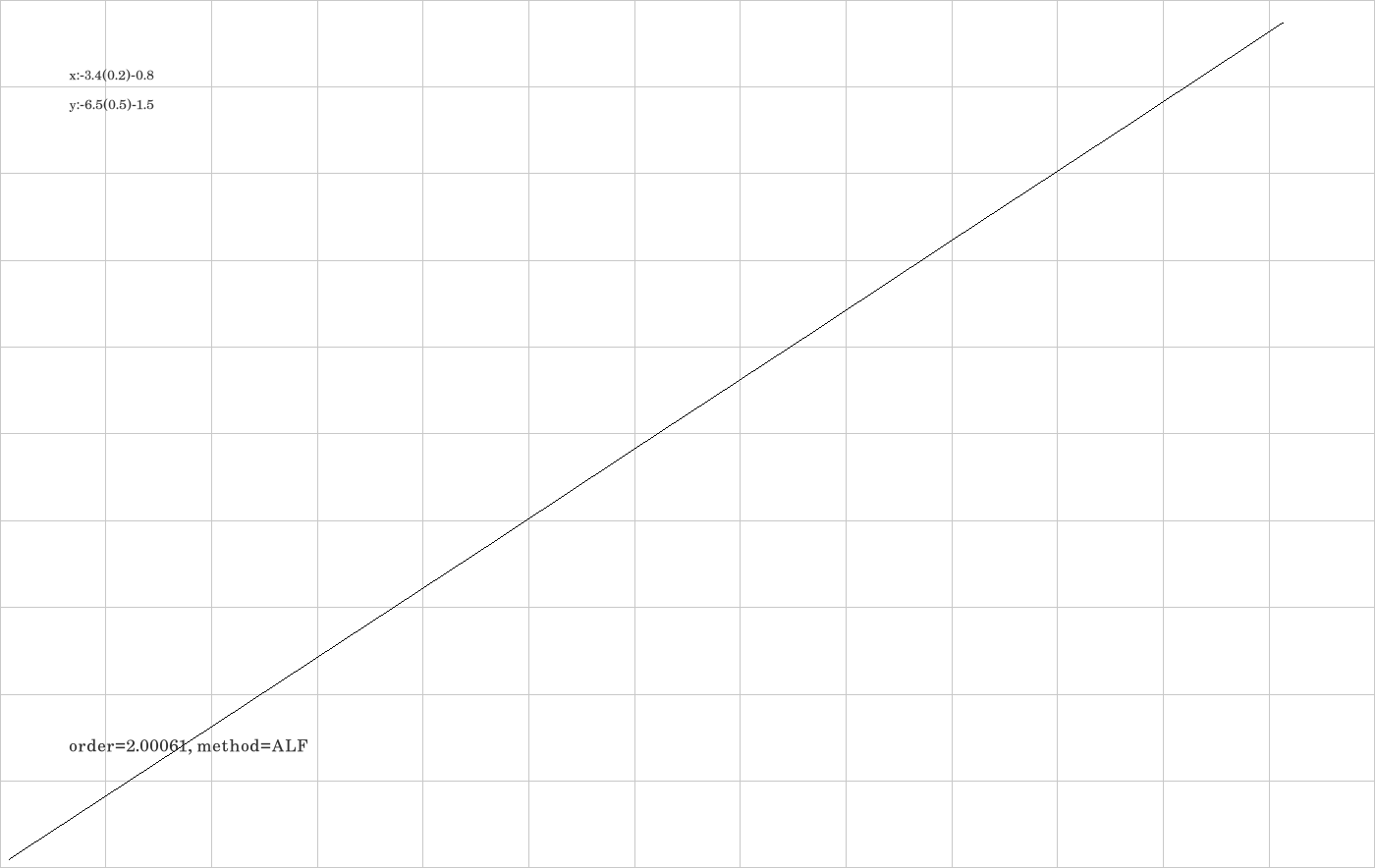
G.2. Empirical order of the ALF-integrator
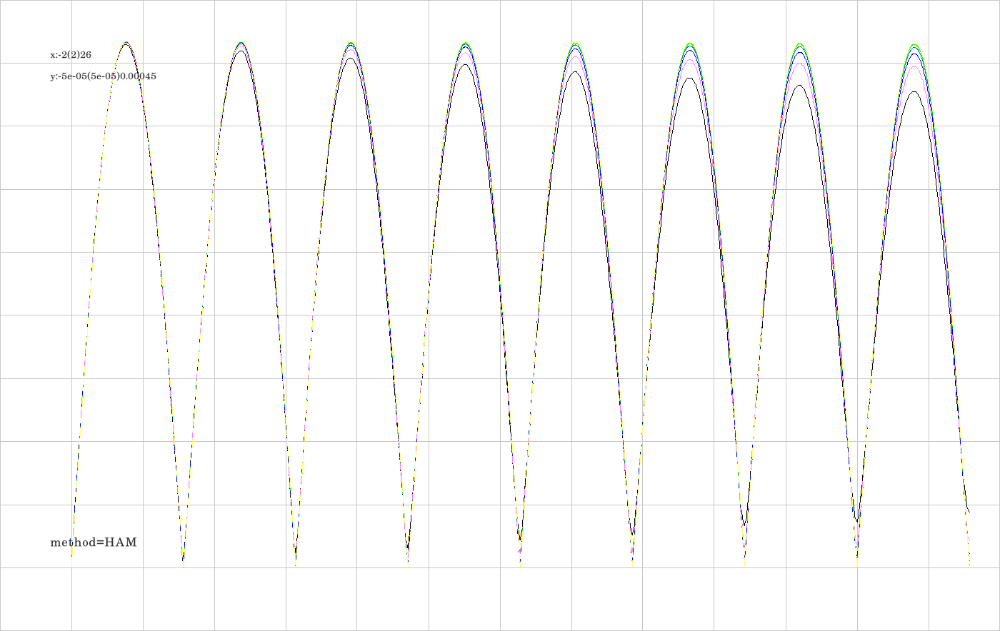
H.1. Position error of first order integrator HAM not perfectly proportional to \(\Delta t\).
H.2. Position error of second order integrator DALF perfectly proportional to \({\Delta t}^2\)
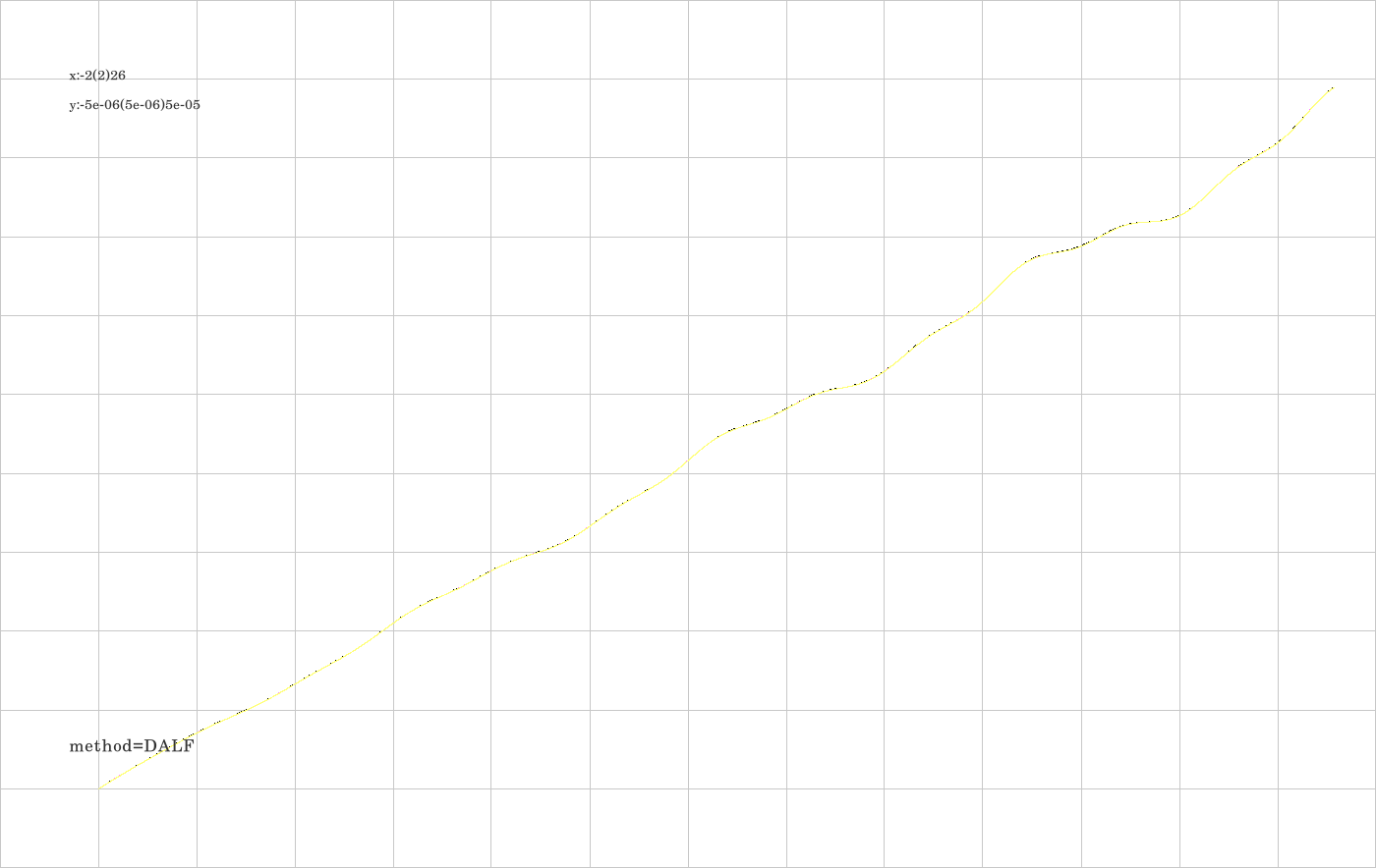
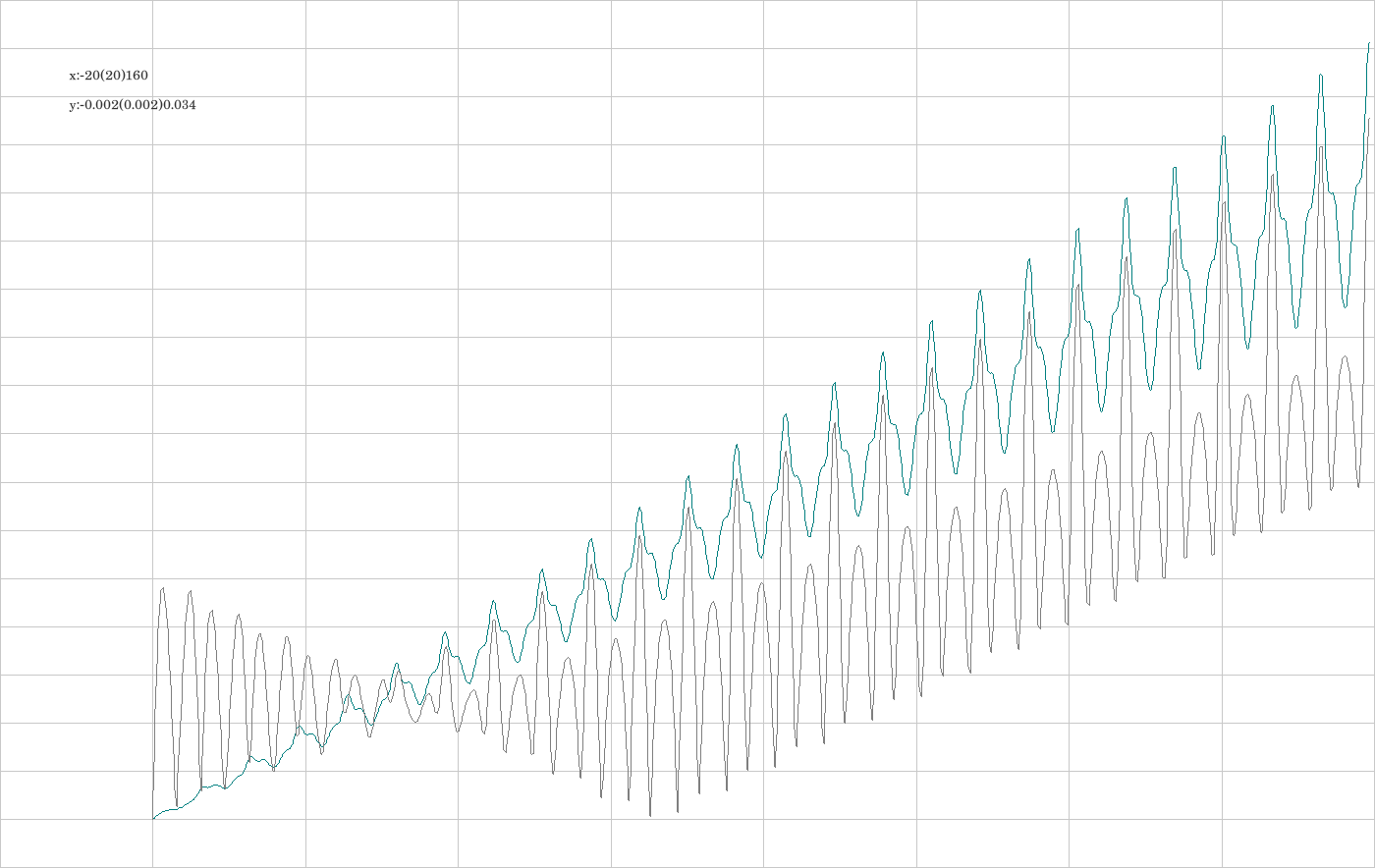
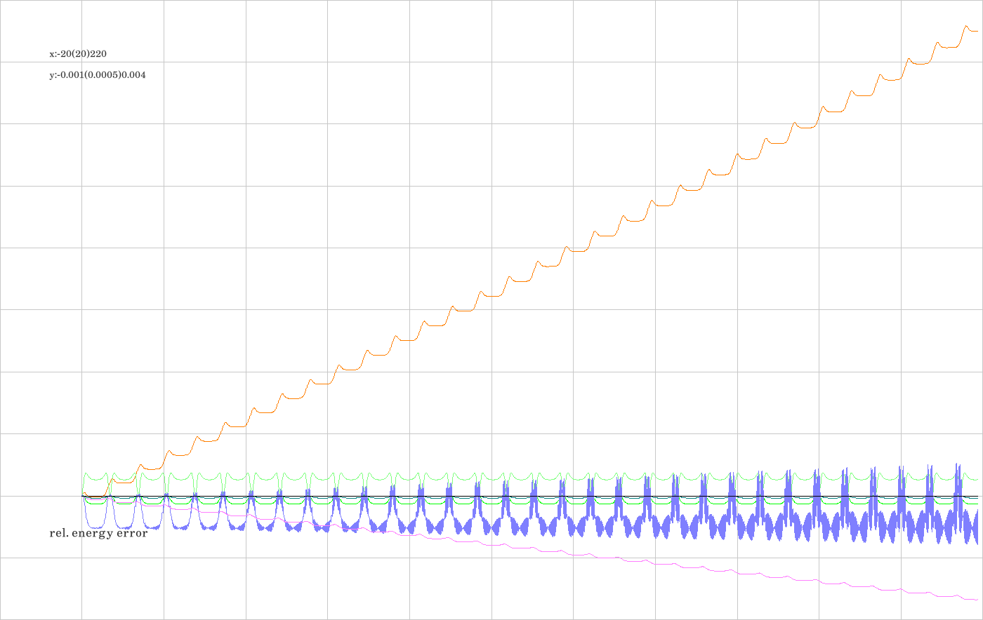
The property which showed up in image A.1., namely that the integrators let the oscillator tick slightly faster than it corresponds to the exact oscillation is shown here for all integrators under consideration.
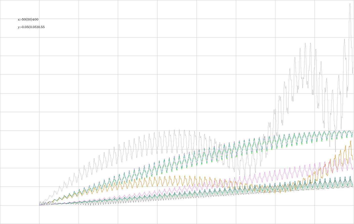
I.1. All integrators over an extended time span
I.2. Some of the integrators over a restricted time span
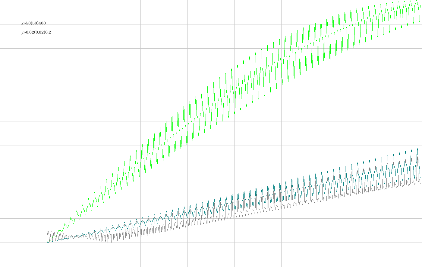
I.3. Some of the integrators over a more restricted time span
These computing tools were used: CPU 4.464 GHz; RAM 16 GB; OS Ubuntu; SW C++20, OpenGL, FreeGlut, Eigen3, Code::Blocks, ffmpeg (for video creation from ppm-files), C+- (self-made C++ library); Compiler GNU.