There is a bundle of motivations behind the present project. First of all, my intention was to to give the asynchronous leapfrog (ALF) method a representation in computer software which is convenient to use in full generality. Very well suited to this endeavor is the programming language C++20. Here the features of templates and of concepts allow a concise description of the conditions under which the ALF-algorithm works.
As to full generality: Since quantum dynamics with a time-independent Hamiltonian is in a sense trivial: the time evolution operator is 'simply' given as the exponential function of an imaginary multiple of the Hamilton operator, we strive for the more ambitious case of a time-dependent Hamiltonian.
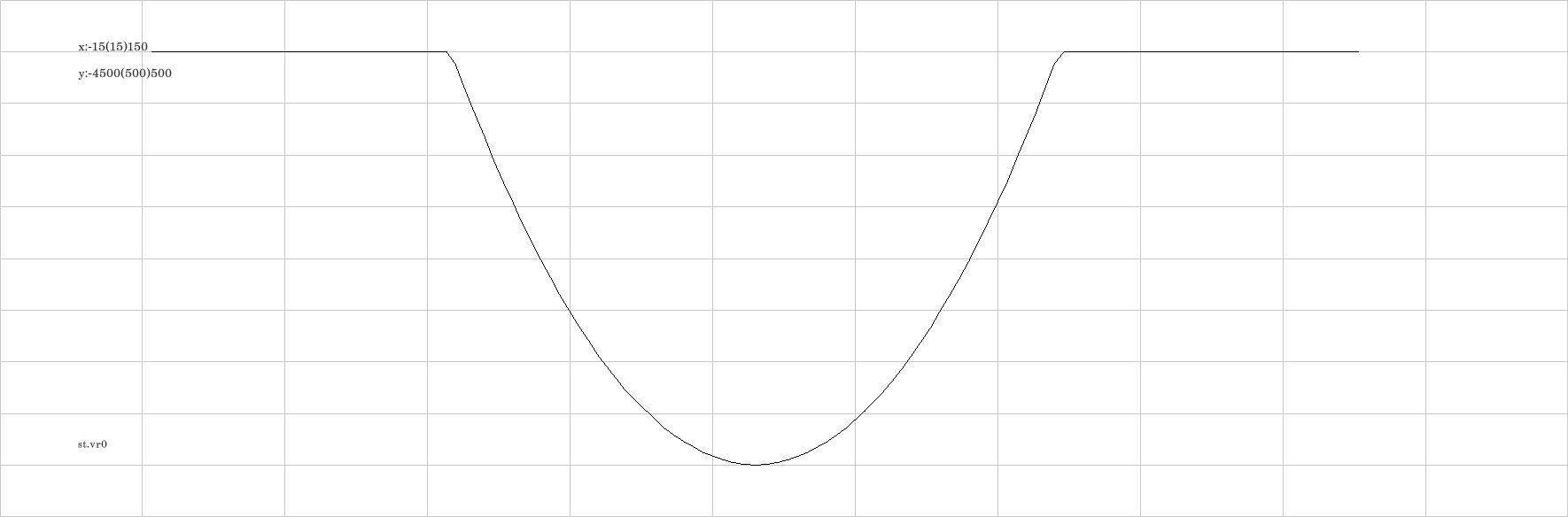
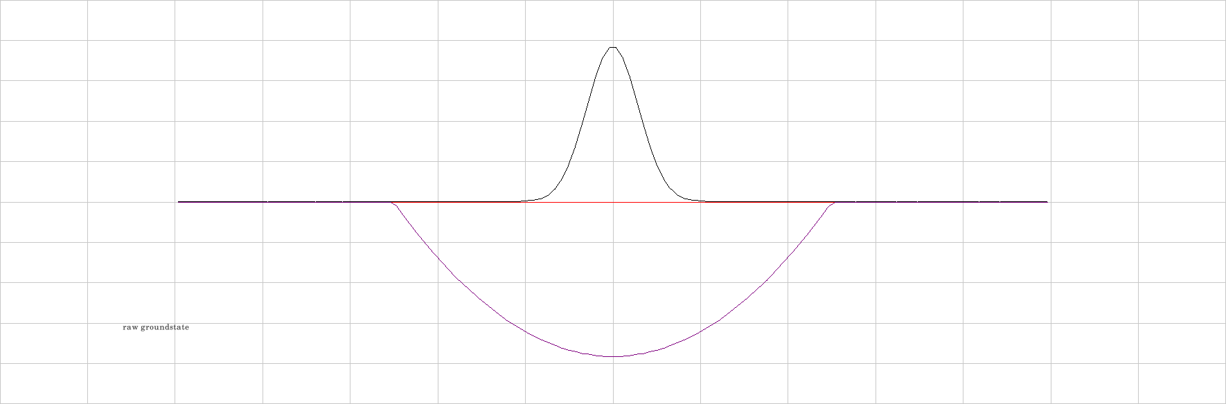
To be specific: we consider a charged quantum particle which is subject to a time-dependent electrical potential. We start with a constant (time-wise) localized attractive potential which holds the particle in place. As in most of our simulations of quantum particle dynamics the particle moves along a finite discrete 1-dimensional biotope. The potential is taken as a parabolic depression below the zero level. The ground-state wave function fills only the deepest part of the potential depression. Let's first have a look on one of the simulation videos and ignore the five 'still images' at the end.
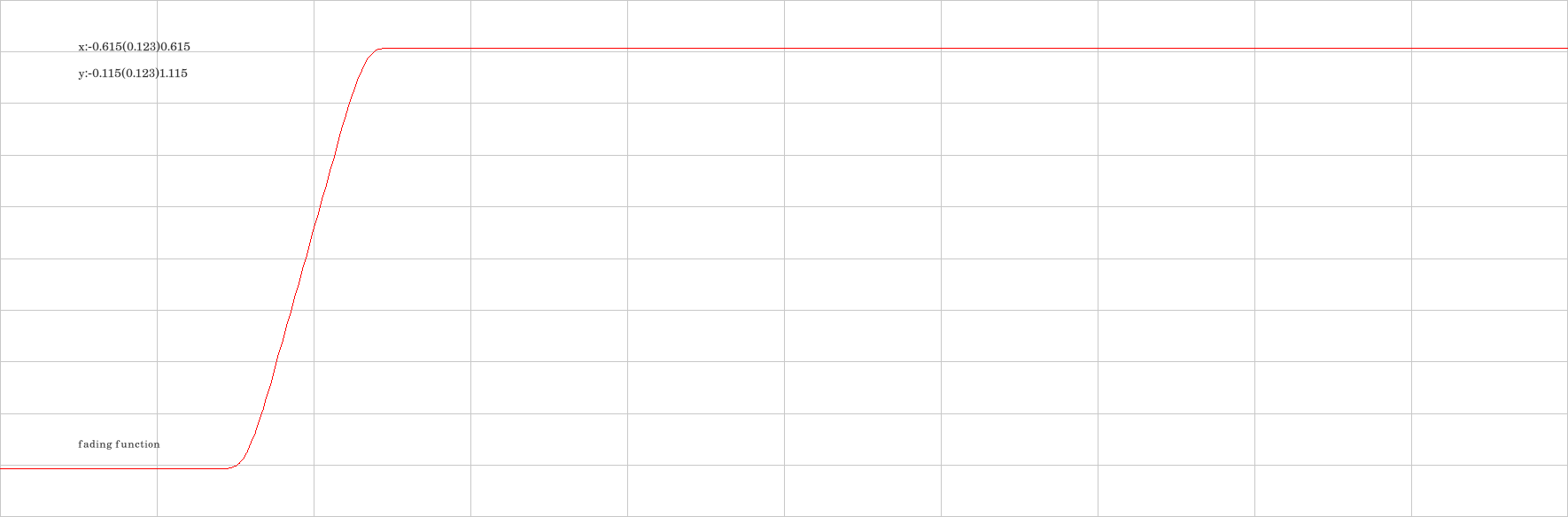
We see the ground state remain constant up to multiplication with a time-dependent imaginary number (the absolute value of the wave function, shown in black, does not change). After a while we observe changes at the left hand side of the potential curve (drawn in magenta). The changes consist in extinguishing the potential from left to right. The mechanism behind this is the following. The potential becomes multiplied by the function which smoothly grows from 0 to 1. What is shown here is the position of the curve at the beginning of the simulation. During the simulation the position of the transition zone moves with constant speed to the right and thus sets to zero larger and larger parts of the potential curve.
During the final disappearance of the potential the automatic time step adjustment increases the step considerably and makes a quick motion effect. Now let us look at some graphics created together with the video showing how the wave function of our particle changes with time. These graphics are appended as kind of still images to the video and could be inspected by stopping the video. A more convenient way is to click the following five pairs of links.
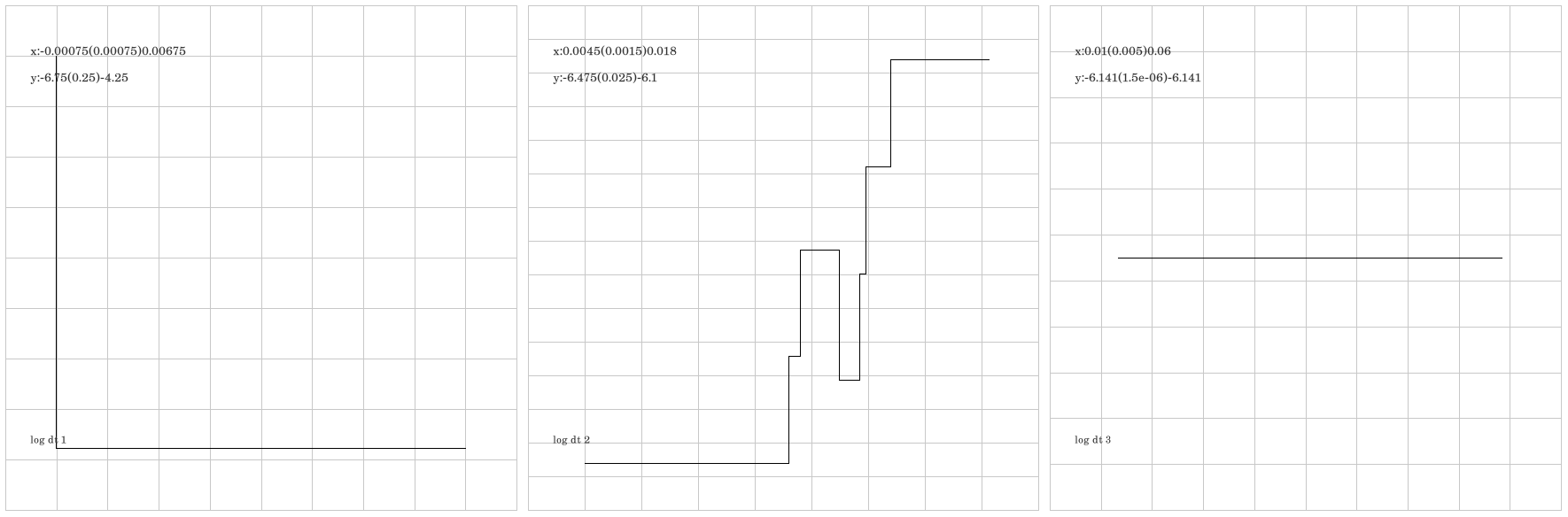
The following explanation is valid for all these links. These links come in pairs: the first with floating point numbers represented as standard type double (i.e. kind of 16 decimal digits), and the second one using boost::multiprecision for 64 decimal digits instead. I added the second version since I was not always sure whether a curve showed mere numerical noise or revealed real substructure. Having for a long time not worked with boost::multiprecision I was surprised that it took only a few code changes to compile with option -pedantic and no warnings. It turned out, however that this holds only if one does not link to the library 'Eigen'. I did'nt need Eigen for my first version of this simulation, in which the Hamiltonoperator was a 128 times 128 matrix. In this case the 64 digit version took only 7% longer to run than the 16 digit version. Bringing Eigen into the game (for avoiding for objectionably slow spectral decomposition of the Hamiltonian) asked for the compilation option -fpermissive and the 7% grew to 22% which is still much less than my expectation coming from experiences from two years ago. As described already the simulation falls into three phases:
1. The potential does not change,
2. the potential fades away till it vanishes in the whole biotope,
3. the potential is gone and the particle moves freely.
To each of these phases we have a separate graphics with separate scale. This is necessary if one doesn't wish to loose the fine structure of the curves due to the limited graphical resolution. Notice that the scale is fully described in the legend near the left upper corner of the graphics. The self-explanatory notation of numerical ranges and subdivisions is taken from the 'Handbook of Mathematical Functions ...' by Abramowitz/Stegun, p.1. Of course, the letters x and y in the legend refer in the traditional way to the horizontal and to the vertical axis and not to the displayed quantities (e.g. time and energy. Near the lower left corner there is a abbreviated hint) to the quantity under consideration.
Read the above two links as a headline to the following paragraph and all the folowing pairs of links the same way.
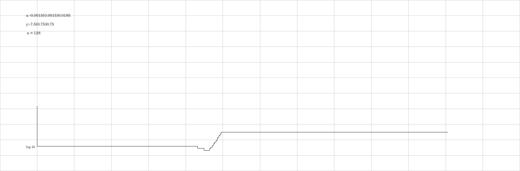
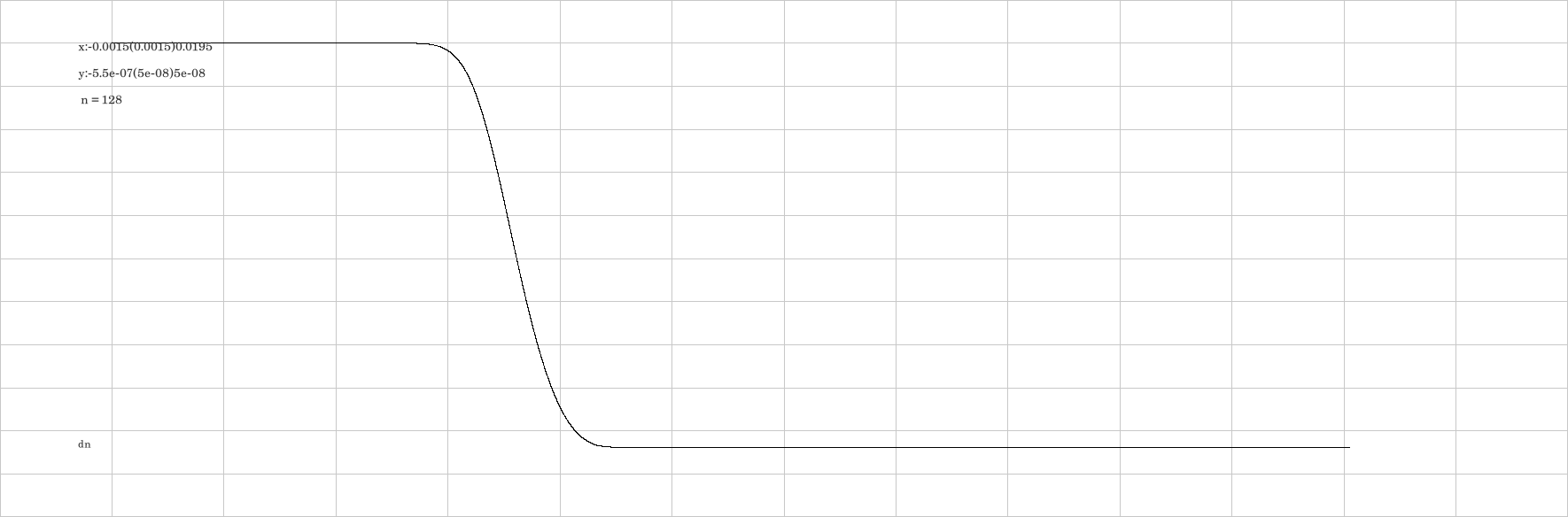
As mentioned already the wave function dynamics is created using the ALF integrator in the mode of automatic time step adjustment. At the beginning of phase 1 the vertical part of the curve indicates that the quite carelessly set initial value 10^-3 for dt was diminished automatically to a working value. This value then was maintained over the whole of phase 1. During phase 2 the weakening of the potential necessitates changes of the time step. The final value from phase 2 can be maintained throughout phase 3. A non dissected logdt-curve (from a simulation with different values of the parameters) is shown here.
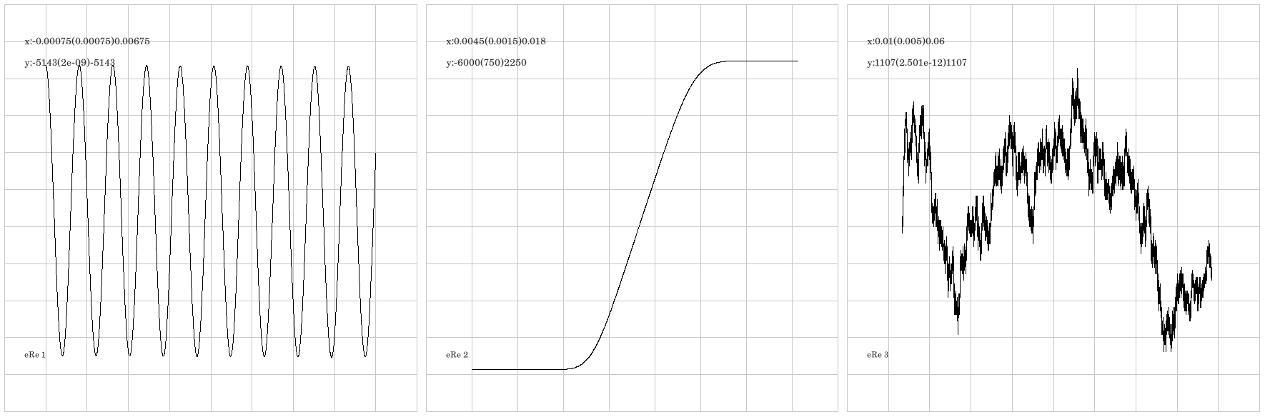
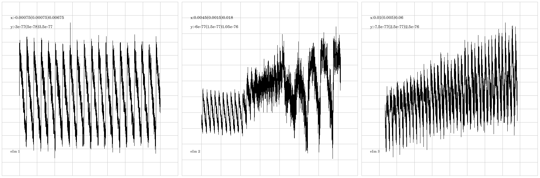
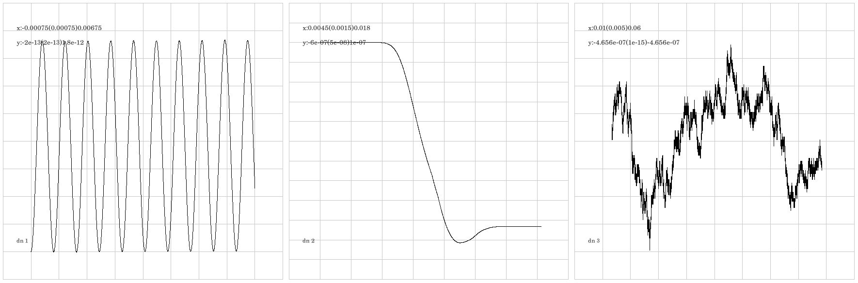
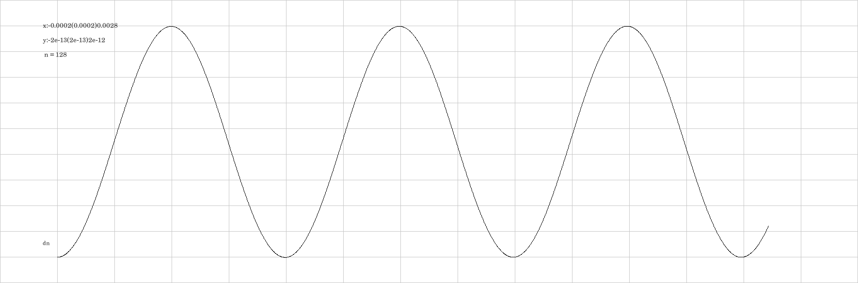
This diagram shows the evolution of the particle energy (i.e. the expectation value of the time-dependent Hamilton operator with respect to the time-dependent state vector in the course of time). If, as is the case here, we use the ALF method to solve the Schroedinger equation, the expectation value of the Hamilton operator can be defined in more than one way. In any case it has to be defined as an expression depending on the dynamical variables ψ and φ, see equation (26) in this article. In a time stepping algorithm it looks natural to use the values which these dynamical variables take at the end of the step as the right input to the energy expression. The ALF algorithm suggest a second option in form of the mid-point state ψ' and φ' in the equation cited above. If we take this option (which I unfortunately not considered earlier) we do not need a second evaluation of the Hamiltonian if we want every time step to output also an energy value. It is encouraging that thus arguments of computational simplicity (no second evaluation of the Hamiltonian) force us to have the energy value associated with the mid-point time t' which slightly differs from the time t. This looks like a hint to the time-energy uncertainty. If the Hamilton operator is hermitian (as it should be and actually is) the expectation value of the energy is rigorously real and in a simulation its imaginary part vanishes up to numerical noise. To double check this fact the energy graphics will later show also the imaginary part of the computed energy.
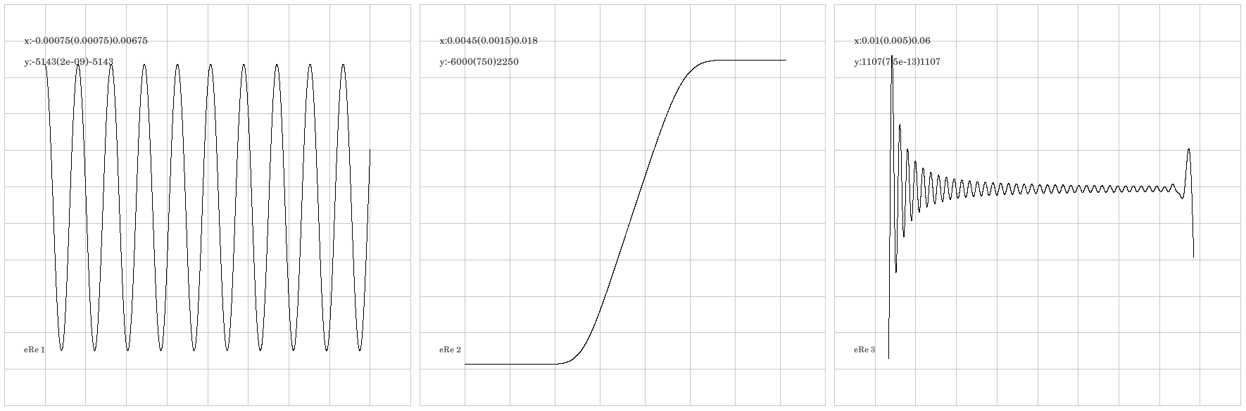
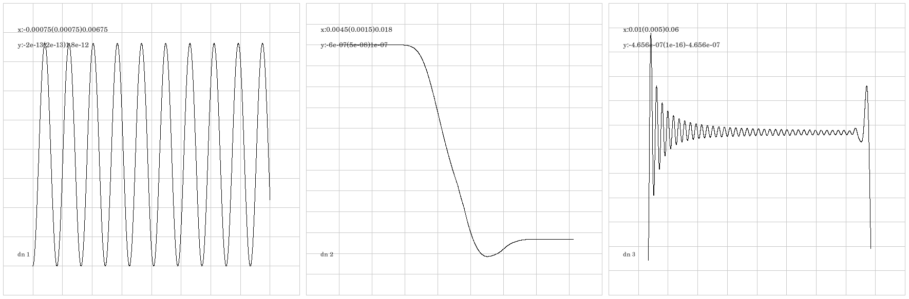
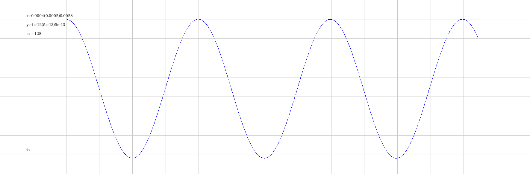
In phase 1 the energy is an eigen value of the Hamiltonian and could be expected to be constant in time. What the graphics shows is a harmonic oscillation with a tiny constant amplitude around a constant location. This is an artifact of the ALF method. The amplitude turns out to be proportional to the square of the time step, so that energy conservation (for time-independent Hamiltonians) holds in the limit of vanishing time step. I tend to speak of pseudo conservation of energy in this case. In phase 2 we see the energy increasing. This is to be expected since the negative potential energy goes to zero in this phase. In phase 3 we again expect constant energy and get a tiny deviation from it as we saw in phase 1. However the pattern is less regular and by three orders of magnitudes smaller. It is obviously affected by numerical noise and is hardly possible to get a convincing idea about the underlying noise-free signal. This is a first occasion for the precision 64 digits version to show its value. Here we see a well-defined curve which apart from front-end and back-end shows pseudo-conservation of energy just as in the case of phase1. Only the amplitude of the oscillation much smaller now. The structure at the back-end it typical for what happens when a free wave meets the rim of its biotope. The structure at the front-end is an artifact from the cut between phase 2 and 3.
Here it looks like one could not say with certainty that this all would be numerical noise. The multiprecision run clearly says that it is.
An other case in which the ALF integrator, when applied to quantum dynamics, gives residual deviations from exact dynamics is pseudo-conservation of norm of the state. In the previous representation of norm minus 1 over the whole time range, the norm change during the transition range (during which the potential changes with time), though tiny, is large enough to hide these residual deviations of the norm from constancy. It becomes visible when we represent it e.g. for the first phase of the simulation. Over the same time range the residual non-constancy of energy shows a closely related pattern. Notice that the amplitudes are only about three orders of magnitude above numerical noise.
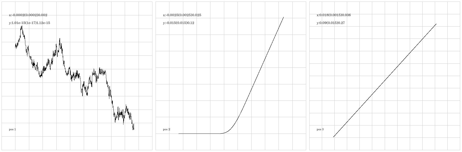
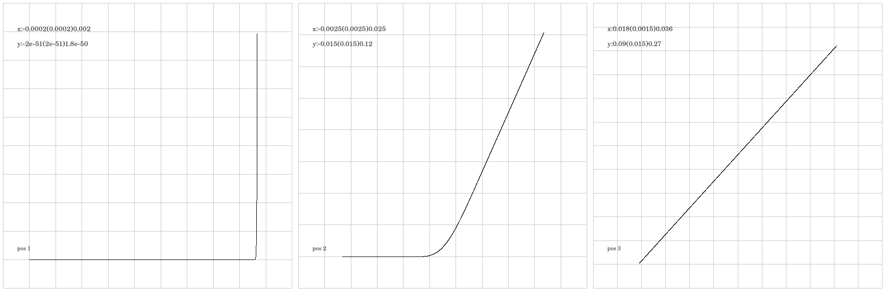
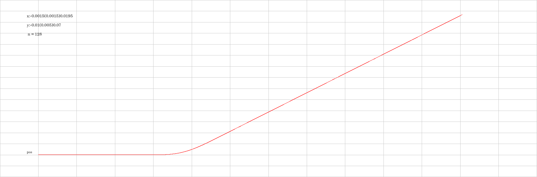
The position of the initial state should be constant in phase 1, should start to move in phase 2, and should grow linearly with time in phase 3. Only the multiprecision-run shows the constant position of the stationary state clearly. See position 64.
During about the second half of its evolution the wave function of the particle shows a free motion with a constant velocity. The graphics concerning the mean position shows this. The cause for this motion of the particle (which was at rest initially) is the our asymmetrical way to switch the potential off.
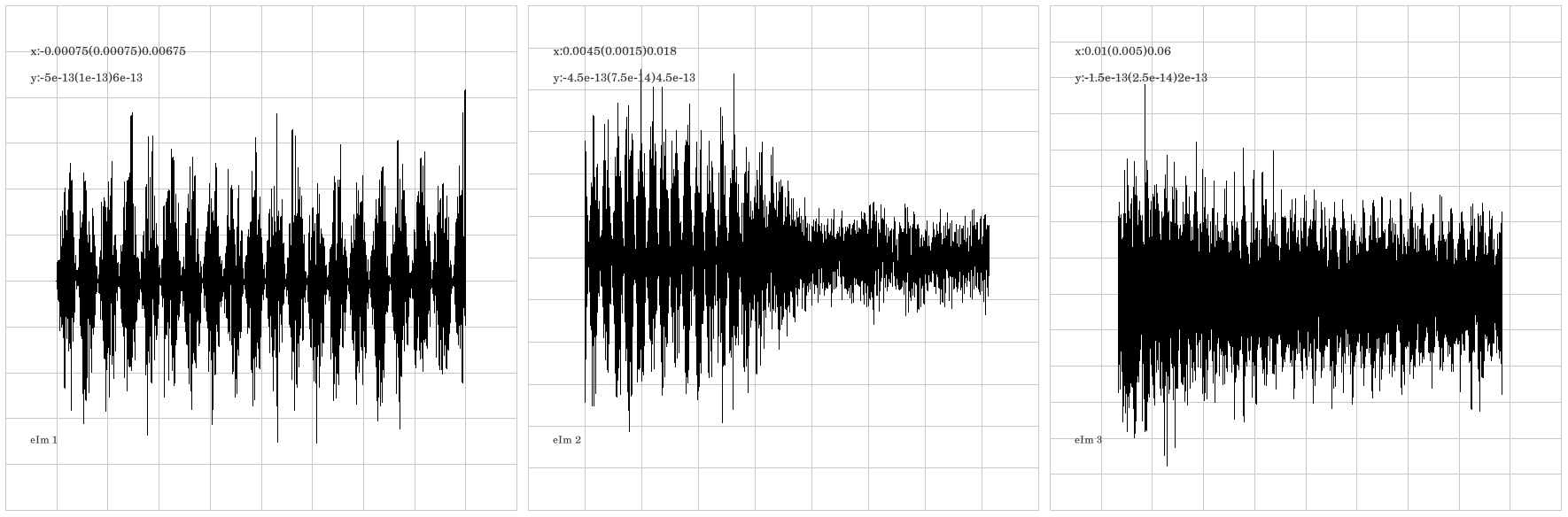
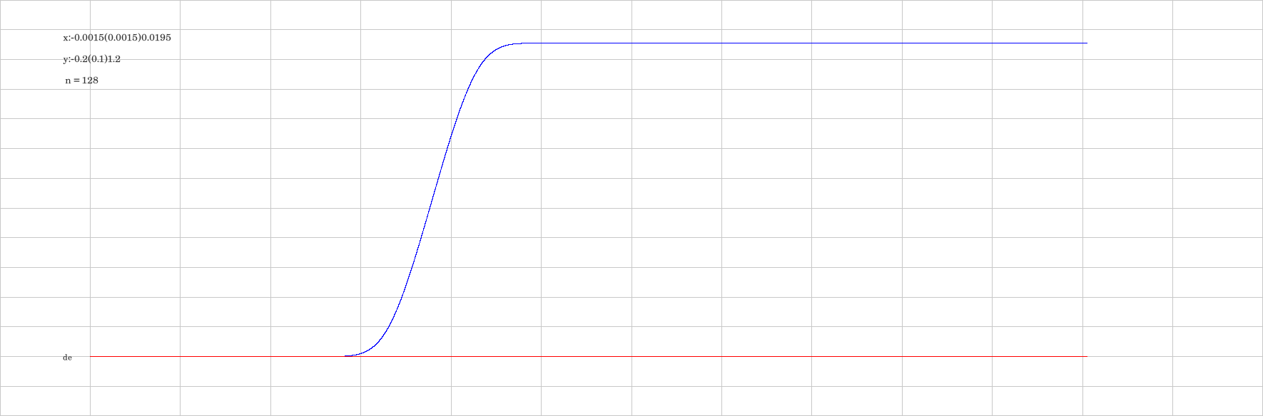
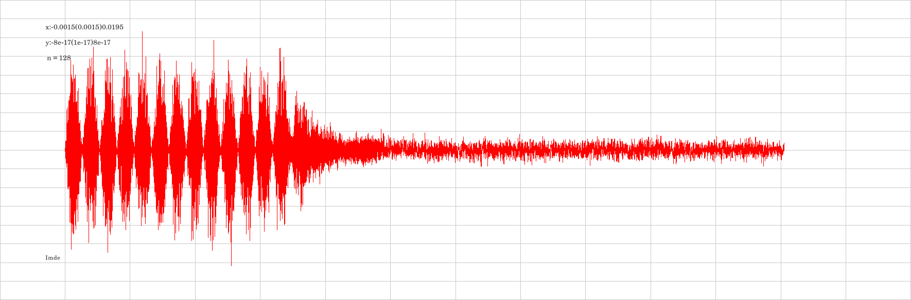
In the process under consideration a bound state with negative energy ends up as a freely moving particle, which obviously has positive energy. It is clear that energy was transferred to the particle by switching off the potential. This is shown by the energy graphics in which the zero-level is chosen as the energy of the initial state. The real part of the total energy of the particle is shown as a blue curve and the imaginary part as a red line. The ALF integrator gives tiny values for the imaginary part of the expectation value of energy. These are too small to be noticeable in the given graphical resolution. If we show it in insulation we see that it is in the order of magnitude of numerical noise but nevertheless shows different patterns for the phases with and without potential.
An other case in which the ALF integrator, when applied to quantum dynamics, gives residual deviations from exact dynamics is pseudo-conservation of norm of the state. In the previous representation of norm-1 over the whole time range, the norm change during the transition range (during which the potential changes with time), though tiny, is large enough to hide these residual deviations of the norm from constancy. It becomes visible when we represent it e.g. for the first phase of the simulation. Over the same time range the residual non-constancy of energy shows a closely related pattern. Notice that the amplitudes are only about three orders of magnitude above numerical noise.
Beside the video above there were created 5 further versions showing ever increasing speed of the fading. The intention behind this was to see how the final energy of the particle depends on the fading speed. From these further videos we have a look only to the last one:
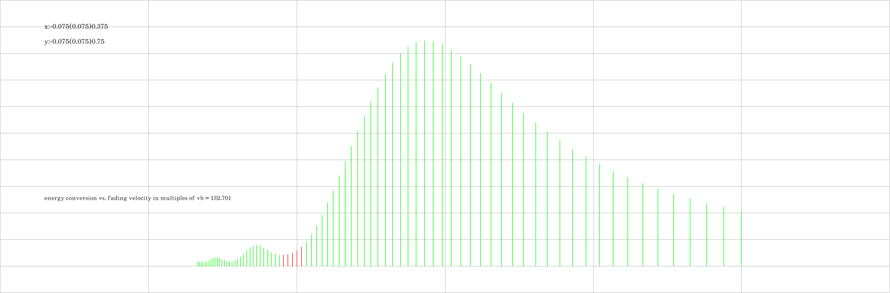
The similarity between all of these six videos (from which only the first and the last one are shown here) suggested that after the vanishing of the potential the particle would run always to the right side and that the final energy would be some fraction (referred to as energy conversion) of the initial binding energy and that this fraction would depend on the fading speed as in quite a featureless way (e.g. close to linear). This expectation turned out to be far from correct when I extended my experimentation to smaller fading speeds. After the first observation of un-expected results I decided to study the situation systematically. The result is this diagram of energy conversion versus fading speed.
Here each vertical line signifies a value of the energy conversion for a value of the fading speed (see legend). If the mean momentum of the particle is positive at the end of the simulation (so the particle tends to run to the right) the line is colored green. If the particle tends to run to the left (the 'irregular case') the color is red.
For one of these red lines (actually the second largest, at x=0.075) the whole evolution is shown (with all parameter except of the fading speed having the same values as in the two previous videos):
Be warned: the first part of the video is a bit dull since it shows for a long while the regular oscillation of the ground state wave function. But when the potential well faded away, the wave function not simply moves to the left side (as one could conclude from the negative sign of the expectation value of the momentum operator) but it splits in a sense into two wave packets which move in different directions. That the left-running part is a bit more 'intensive' than the right-running one is not at all obvious from the video representation of the wave function.
These are the miracles of quantum mechanics: If we would realize with good semiconductor engineering our 'triggerable one electron gun' and would let it fire millions of times, we would find the detected electrons distributed according to the square of the absolute value of the wave function which the Alf algorithm was able to deliver with relative ease.
These computing tools were used: CPU 4.464 GHz; RAM 16 GB; OS Ubuntu; SW C++20, boost::multiprecision, OpenGL, FreeGlut, Code::Blocks, ffmpeg (for video creation from ppm-files), pnmtopng (for conversion from ppm to png), C+- (a self-made C++ library); Compiler GNU.